H. Paul Keeler

Voronoi tessellations

Cholera outbreaks due to public water pumps. Suburbs serviced by hospitals. Formation of crystals. Coverage regions of phone towers. We can model or approximate all these phenomena and many, many more with a geometric structure called, among other names, a Voronoi tessellation.

To form a Voronoi tessellation, consider a collection of points scattered on some space, like the plane, where it’s easier to picture things, especially when using a Euclidean metric. Now for each point in the collection, consider the surrounding region that is closer to that point than any other point in the collection. Each region forms a cell corresponding to the point. The union of all the sets covers the underlying space. That union of sets is the Voronoi tessellation.

The evolution of Voronoi cells, which start off as disks until they collide with each other. Source: Wikipedia.

Mathematicians have extensively studied Voronoi tessellations, particularly those based on Poisson point processes, forming a core subject in the field of stochastic geometry.

It’s also called a Dirichlet tessellation

The main other name for the Voronoi tessellation is the Dirichlet tessellation. Historically, Dirichlet beats Voronoi, but it seems wherever I look, the name Voronoi usually wins out, suggesting an example of Stigler’s law of eponymy. A notable exception is the R library spatstat that does actually call it a Dirichlet tessellation. Wikipedia calls it a Voronoi diagram. I’ve read that Descartes studied the object even earlier than Dirichlet, but Voronoi studied it in much more depth. At any rate, I will call it a Voronoi tessellation.

Everyday Voronoi tessellations

Voronoi tessellations are just not interesting mathematical objects, as they arise in everyday situations. This piece from Scientific American website explains:

Everyone uses Voronoi tessellations, even without realizing it. Individuals seeking the nearest café, urban planners determining service area for hospitals, and regional planners outlining school districts all consider Voronoi tessellations. Each café, school, or hospital is a site from which a Voronoi tessellation is generated. The cells represent ideal service areas for individual businesses, schools, or hospitals to minimize clientele transit time. Coffee drinkers, patients, or students inside a service area (that is, a cell) should live closer to their own café, hospital, or school (that is, their own cell’s site) than any other. Voronoi tessellations are ubiquitous, yet often invisible.

Delaunay triangulation

A closely related object is the Delaunay triangulation. For a given collection of points on some underlying mathematical space, a Delaunay triangulation is formed by connecting the points and creating triangles with the condition that for each point, no other point exists in the circumcircle of the corresponding triangle. (A circumcircle is a circle that passes through all three vertices of a triangle.)

The vertices of the the Delaunay triangular and Voronoi tessellation both form graphs, which turn out to be the dual graphs of each other.

A Delaunay triangulation (in black) and the corresponding Voronoi tessellation (in red) whose vertices are the centres of the circumcircles of the Delaunay triangles. Source: Wikipedia.

Software: Qhull

Due to its applications, it’s not surprising that there exist algorithms that quickly create or estimate Voronoi tessellations. I don’t want to implement one of these algorithms from scratch, as they have already been implemented in various scientific programming languages. Many of the languages, such as MATLAB, R, and Python (SciPy) use the code from Qhull. (Note the Qhull website calls the tessellation a Voronoi diagram.)

(The Julia programming language, which I examined in a previous post, has a Voronoi package that does not use Qhull.)

Qhull finds the Voronoi tessellation by first finding the Delaunay triangulation. If the underlying space is bounded, then all the Voronoi cells are also bounded. But on an unbounded space, it is possible to have unbounded cells, meaning their areas (or volumes) are infinite. In such cases, the algorithms sometime place virtual points at infinity, but I don’t want to focus on such details. I will assume Qhull does a good job.

Code

As always, the code from all my posts is online. For this post, the MATLAB and Python code is here and here, respectively, which generates Voronoi tesselations.

MATLAB

It is fairly straightforward to create Voronoi tessellations in MATLAB. You can just use the function voronoi, which is only for two-dimensional tessellations. (Note: the MATLAB website says the behaviour of the function voronoi has changed, so that may cause problems when using different versions of MATLAB.) The function requires two inputs as vectors, say, x and y, corresponding to the Cartesian (or $x$ and $y$) coordinates of the points. If you just run the voronoi command, it will create and plot a Voronoi tessellation (or Voronoi diagram, as MATLAB calls it). But the MATLAB website also describes how to plot the tessellation manually.

For $d$ -dimensional tessellations, there is the function voronoin, which requires a single input. The single output consists of combining $d$ column vectors for the Cartesian coordinates. For example, given the column vectors x, y and z, then the input is [x, y, z].

If you give the functions voronoi or voronoin output arguments, then the tessellation is not plotted and instead two data structures, say, v and c are created for describing the vertices of the tessellation. I generally use voronoi for plotting, but I use voronoin (and not voronoi) for generating vertex data, so I will focus on the outputs of voronoin.

For voronoin, the first (output) data structure v is simply an two-dimensional array array that contain the Cartesian coordinates of every vertex in the Voronoi tessellation. The second (output) data structure c is a cell array describing the vertices of each Voronoi cell (it has to be a cell array, as opposed to a regular array, as the cells have varying number of vertices). Each entry of the cell array contains a one-dimensional array with array indices corresponding to the $x$ and $y$ coordinates.

The code checks which Voronoi cells are unbounded by seeing if they have vertices at infinity, which corresponds to a $1$ in the index arrays (stored in the structure array c).

One criticism of the MATLAB functions is that they don’t return all the information of the Voronoi tessellation. More specifically, the functions don’t return the boundaries between the unbounded cells, though voronoi internally calculates and uses these boundaries to generate Voronoi plots. This is covered in this review on different Voronoi packages. Conversely, the Python package returns more information such as that of the edges or ridges of the Voronoi cells.

Python

To create the Voronoi tessellation, use the SciPy (Spatial) function Voronoi. This function does $d$-dimensional tessellations. For the two-dimensional setting, you need to input the $x$ and $y$ coordinates as a single array of dimensions $2 \times n$, where $n$ is the number of points in the collection. In my code, I start off with two one-dimensional arrays for the Cartesian coordinates, but then I combined them into a single array by using the function numpy.stack with the function argument axis =1.

I would argue that the Voronoi function in SciPy is not as intuitive to use as the MATLAB version. One thing I found a bit tricky, at first, is that the cells and the points have a different sets of numbering (that is, they are indexed differently). (And I am not the only one that was caught by this.) You must use the attribute called point_region to access a cell number (or index) from a point number (or index). In my code the attribute is accessed and then called it indexP2C, which is an integer array with cell indices. Of course, there could be a reason for this, and I am just failing to understand it.

Apart from the above criticism, the function Voronoi worked well. As I mentioned before, this package returns more Voronoi information than the MATLAB equivalents.

To plot the Voronoi tessellation, use the SciPy function voronoi_plot_2d, which allows for various plotting options, but it does require Matplotlib. The input is the data object created by the function Voronoi.

Results

I’ve plotted the results for a single realization of a Poisson point process. I’ve also plotted the indices of the points. Recall that the indexing in Python and MATLAB start respectively at zero and one.

MATLAB

Python

Voronoi animations

I took the animation of evolving Voronoi cells, which appears in the introduction, from Wikipedia. The creator generated it in MATLAB and also posted the code online. The code is long, and I wouldn’t even dare to try to reproduce it, but I am glad someone else wrote it.

Such animations exist also for other metrics. For example, the Manhattan metric (or taxi cab or city block metric) gives the animation below, where the growing disks have been replaced with squares.

A Voronoi tessellation under the Manhattan metric. The evolving cells start off as squares until they collide with each other. Source: Wikipedia.

This Wikipedia user page has animations under other metrics on Euclidean space.

This post also features animations of Voronoi tessellations when the points move.

Simulating a Cox point process based on a Poisson line process

In the previous post, I described how to simulate a Poisson line process, which in turn was done by using insight from an earlier post on the Bertrand paradox.

Now, given a Poisson line process, for each line, if we generate an independent one-dimensional Poisson point point process on each line, then we obtain an example of a Cox point process. Cox point processes are also known as doubly stochastic Poisson point processes. On the topic of names, Guttorp and Thorarinsdottir argue that it should be called the Quenouille point process, as Maurice Quenouille introduced an example of it before Sir David Cox, but I opt for the more common name.

Cox point proceesses

A Cox point process is a generalization of a Poisson point process. It is created by first considering a non-negative random measure, sometimes called a driving measure. Then a Poisson point process, which is independent of the random driving measure, is generated by using the random measure as its intensity or mean measure.

The driving measure of a Cox point process can be, for example, a non-negative random variable or field multiplied by a Lebesgue measure. In our case, the random measure is the underlying Poisson line process coupled with the Lebesgue measure on the line (that is, length).

Cox processes form a very large and general family of point processes, which exhibit clustering. In previous posts, I have covered two special cases of Cox point processes: the Matérn and Thomas cluster point processes. These are, more specifically, examples of a Neyman-Scott point process, which is a special case of a shot noise Cox point process. These two point processes are fairly easy to simulate, but that’s not the case for Cox point processes in general. Some are considerably easier than others.

Motivation

I will focus on simulating the Cox point process formed from a Poisson line process with homogeneous Poisson point processes. I do this for two reasons. First, it’s easy to simulate, given we can simulate a Poisson line process. Second, it has been used and studied recently in the mathematics and engineering literature for investigating wireless communication networks in cities, where the streets correspond to Poisson lines; for example, see these two preprints:

Incidentally, I don’t know what to call this particular Cox point process. A Cox line-point process? A Cox-Poisson line-point process? But it doesn’t matter for simulation purposes.

Method

We will simulate the Cox (-Poisson line-) point process on a disk. Why a disk? I suggest reading the previous posts on the Poisson line process and the Bertrand paradox for why the disk is a natural simulation window for line processes.

Provided we can simulate a Poisson line process, the simulation method is quite straightforward, as I have essentially already described it.

Line process

First simulate a Poisson line process on a disk. We recall that for each line of the line process, we need to generate two independent random variables $\Theta$ and $P$ describing the position of the line. The first random variable $\Theta$ gives the line orientation, and it is a uniform random variable on the interval $(0,2\pi)$.

The second random variables $P$ gives the distance from the origin to the disk edge, and it is a uniform random variable on the interval $(0,r)$, where $r$ is the radius of the disk. The distance from the point $(\Theta, P)$ to the disk edge (that is, the circle) along the chord is:

$$Q=\sqrt{r^2-P^2}.$$

The endpoints of the chord (that is, the points on the disk edge) are then:

Point 1: $X_1=P \cos \Theta+ Q\sin \Theta$, $Y_1= P \sin \Theta- Q\cos \Theta$,

Point 2: $X_2=P \cos \Theta- Q\sin \Theta$, $Y_2= P \sin \Theta+Q \cos \Theta$.

The length of the line segment is $2 Q$. We can say this random line is described by the point $(\Theta,P)$.

One-dimensional Poisson point process

For each line (segment) in the line process, simulate a one-dimensional Poisson point process on it. Although I have never discussed how to simulate a one-dimensional (homogeneous) Poisson point process, it’s essentially one dimension less than simulating a homogeneous Poisson point process on a rectangle.

More specifically, given a line segment $(\Theta,P)=(\theta,p)$, you simulate a homogeneous Poisson point process with intensity $\mu$ on a line segment with length $2 q$, where $q=\sqrt{r^2-p^2}$. (I am now using lowercase letters to stress that the line is no longer random.) To simulate the homogeneous Poisson point process, you generate a Poisson random variable with parameter $2 \mu q$.

Now you need to place the points uniformly on the line segment. To do this, consider a single point on a single line. For this point, generate a single uniform variable $U$ on the interval $(-1,1)$. The tricky part is now getting the Cartesian coordinates right. But the above expressions for the endpoints suggest that the single random point has the Cartesian coordinates:

$x=p \cos \theta+ U q\sin \theta$, $y=p \sin \theta- U q\cos \theta$.

The two extreme cases of the uniform random variable $U$ (that is, $U=-1$ and $U=1$) correspond to the two endpoints of the line segment. We recall that $Q$ is the distance from the midpoint of the line segment to the disk edge along the line segment, so it makes sense that we want to vary this distance uniformly in order to uniformly place a point on the line segment. This uniform placement step is done for all the points of the homogeneous Point process on that line segment.

You repeat this procedure for every line segment. And that’s it: a Cox point process built upon a Poisson line process.

Results

MATLAB

R

Python

Code

As always, the code from all my posts is online. For this post, I have written the code in MATLAB, R and Python.

Simulating a Poisson line process

Instead of points, we can consider other objects randomly scattered on some underlying mathematical space. If we take a Poisson point process, then we can use (infinitely long) straight lines instead of points, giving a Poisson line process. Researchers have studied and used this random object to model physical phenomena. In this post I’ll cover how to simulate a homogeneous Poisson line process in MATLAB, R and Python. The code can be downloaded from here.

Overview

For simulating a Poisson line process, the key question is how to randomly position the lines. This is related to a classic problem in probability theory called the Bertrand paradox. I discussed this illustration in probability in a previous post, where I also included code for simulating it. I highly recommend reading that post first.

The Bertrand paradox involves three methods for positioning random lines. We use Method 2 to achieve a uniform positioning of lines, meaning the number of lines and orientation of lines is statistically uniform. Then it also makes sense to use this method for simulating a homogeneous (or uniform) Poisson line process.

We can interpret a line process as a point process. For a line process on the plane $\textbf{R}^2$, it can be described by a point process on $(0,\infty)\times (0,2\pi)$, which is an an infinitely long cylinder. In other words, the Poisson line process can be described as a Poisson point process.

For simulating a Poisson line process, it turns out the disk is the most natural setting. (Again, this goes back to the Bertrand paradox.) More specifically, how the (infinitely long) lines intersect a disk of a fixed radius $r>0$. The problem of simulating a Poisson line process reduces to randomly placing chords in a disk. For other simulation windows in the plane, we can always bound any non-circular region with a sufficiently large disk.

Steps

Number of lines

Of course, with all things Poisson, the number of lines will be a Poisson random variable, but what will its parameter be? This homogeneous (or uniform) Poisson line process forms a one-dimensional homogeneous (or uniform) Poisson point process around the edge of the disk with a circumference $2 \pi r $. Then the number of lines is simply a Poisson variable with parameter $\lambda 2 \pi r $.

Locations of points

To position a single line uniformly in a disk, we need to generate two uniform random variables. One random variable gives the angle describing orientation of the line, so it’s a uniform random variable $\Theta$ on the interval $(0,2\pi)$.

The other random variable gives the distance from the origin to the disk edge, meaning it’s a uniform random variable $P$ on the interval $(0,r)$, where $r$ is the radius of the disk. The random radius and its perpendicular chord create a right-angle triangle. The distance from the point $(\Theta, P)$ to the disk edge (that is, the circle) along the chord is:

$$Q=\sqrt{r^2-P^2}.$$

The endpoints of the chord (that is, the points on the disk edge) are then:

Point 1: $X_1=P \cos \Theta+ Q\sin \Theta$, $Y_1= P \sin \Theta- Q\cos \Theta$,

Point 2: $X_2=P \cos \Theta- Q\sin \Theta$, $Y_2= P \sin \Theta+Q \cos \Theta$.

Code

I have implemented the simulation procedure in MATLAB, R and Python, which, as usual, are all very similar. I haven’t put my code here, because the software behind my website keeps mangling it. As always, I have uploaded my code to a repository; for this post, it’s in this directory.

I have written the code in R, but I wouldn’t use it in general. That’s because if you’re using R, then, as I have said before, I strongly recommend using the powerful spatial statistics library spatstat. For a simulating Poisson line process, there’s the function rpoisline.

The chief author of spatstat, Adrian Baddeley, has written various lectures and books on the related topics of point processes, spatial statistics, and geometric probability. In this post, he answered why the angular coordinates have to be chosen uniformly.

Results

MATLAB

Python

Creating a simple feedforward neural network (without using libraries)

Deep learning refers several classes of statistical models, most often neural networks, which are deep in the sense that they have many layers between the input and output. We can think of these layers as computational stages.

(More precisely, you can think of them as very big matrices.)

These statistical models have now become interchangeable with the much loved term artificial intelligence (AI). But how do neural networks work?

Neural networks are collections of large — often extraordinarily large — matrices with values that have been carefully chosen (or found) so that running inputs through these matrices generates accurate outputs for certain problems like classifying photos or writing readable sentences. There are many types of neural networks, but to understand them, it’s best to start with a basic one, which is an approach I covered in a previous post.

Without using any of the neural network libraries in MATLAB or Python (of which there are several), I wrote a simple four-layer feedforward (neural) network, which is also called a multilayer perceptron. This is an unadorned neural network without any of the fancy bells and whistles that they now possess.

And that’s all you need to understand the general gist of deep learning.

Binary classification problem

I applied the simple neural network to the classic problem of binary classification. More specifically, I created a simple problem by divided two-dimensional (Cartesian) square into two non-overlapping regions. My neural network needs to identify in region a point lies in a square. A simple problem, but it is both fundamental and challenging.

I created three such problems with increasing difficulty. Here they are:

Simple: Ten points of two types located in a square, where the classification border between the two types is curve lined.
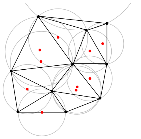
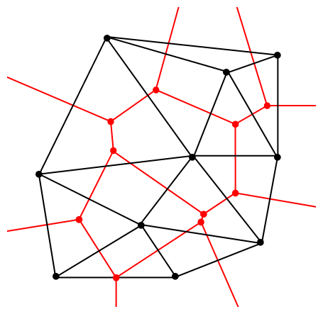
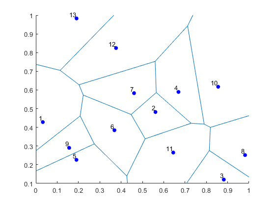
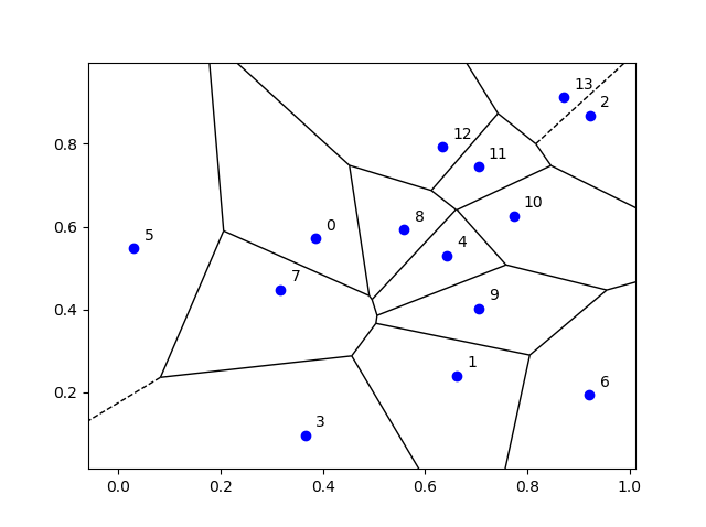
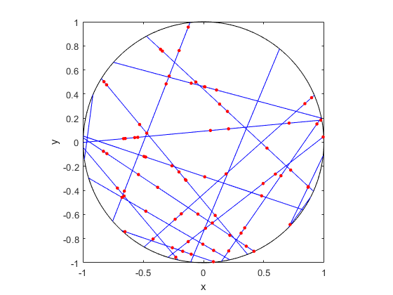
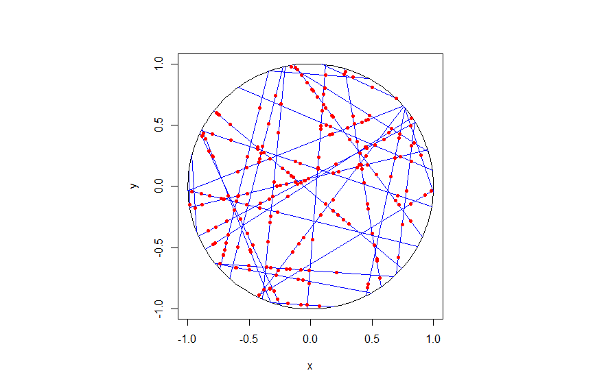
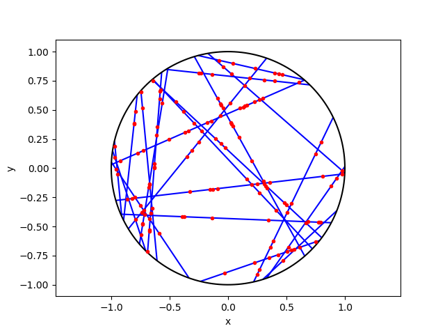
Voronoi: A Voronoi tessellation is (deterministically) created with a small number of seeds (or Voronoi cells). A point can either be in a given Voronoi cell or not, hence there are two types of points.
Rose: A simple diagram of a four-petal flower or rose is created using a polar coordinates. Located entirely inside a square, points can either be inside the rose or not, giving two types of points.

Components of the neural network model

Optimization method

I fitted or or trained my four-layer neural network model by using a simple stochastic gradient descent method. The field of optimization (or operations research) abounds with methods based on gradients (or derivatives), which usually fall under the category of convex optimziation.

In the code I wrote, a random coordinate is chosen, and then the fitting (or optimization) method takes a step where the gradient is the largest, where the size of step is dictated by a fixed constant called a learning rate. This procedure is repeated for some pre-fixed number of steps. The random choosing of the coordinate is done with replacement.

This is basically the simplest training method you can use. In practice, you never use such simple methods, relying upon more complex gradient-based methods such as Adam.

Cost function

For training, the so-called cost function or loss function is a root-mean-square function,¹ which goes against the flow today, as most neural networks now employ cost functions based on the maximum likelihood and cross-entropy. There is a good reason why these are used instead of the root-mean-square. They work much better.

Activation function

For the activation function, the code uses the sigmoid function, but you can easily change it to use recitified linear unit (ReLU), which is what most neural networks use today. For decades, it commonly accepted to use the sigmoid function, partly because it’s smooth. But it seems only work well for small networks. The rectified linear unit reigns supreme now, as it is considerably better than the sigmoid function and others in large neural networks.

Code

I stress that this code is only for educational purposes. It’s designed to gain intuition into how (simple) neural networks do what they do.

If you have a problem that requires neural networks (or deep learning), then use one of the libraries such as PyTorch or TensorFlow. Do not use my code for such problems.

I generally found that the MATLAB code run much faster and smoother than the Python code. Python isn’t great for speed. (Serious libraries are not written in Python but C or, like much of the matrix libraries in Python, Fortran.)

Here’s my code.

MATLAB

% This code runs a simple feedforward neural network inspired.
%
% The neural network is a multi-layer perceptron designed for a simple
% binary classification. The classification is determining whether a
% two-dimensional (Cartesian) point is located inside some given region or
% not.
%
% For the simple binary examples used here, the code seems to work for
% sufficiently large number of optimization steps, typically in the 10s and
% 100s of thousands.
%
% This neural network only has 4 layers (so 2 hidden layers). The
% trainning procedure, meaning the forward and backward passes, are
% hard-coded. This means changing the number of layers requires additional
% information on the neural network architecture.
%
% It uses the sigmoid function; see the activate function.
%
% NOTE: This code is for illustration and educational purposes only. Use a
% industry-level library for real problems.
%
% Author: H. Paul Keeler, 2019.
% Website: hpaulkeeler.com
% Repository: github.com/hpaulkeeler/posts

clearvars; clc; close all;

choiceData=3; %choose 1, 2 or 3
numbSteps = 2e5; %number of steps for the (gradient) optimization method
rateLearn = 0.05; %hyperparameter
numbTest = 1000; %number of points for testing the fitted model
boolePlot=true;

rng(42); %set seed for reproducibility of results

%generating or retrieving the training data
switch choiceData
    case 1
        %%% simple example
        %recommended minimum number of optimization steps: numbSteps = 1e5
        x1 = 2*[0.1,0.3,0.1,0.6,0.4,0.6,0.5,0.9,0.4,0.7]-1;
        x2 = 2*[0.1,0.4,0.5,0.9,0.2,0.3,0.6,0.2,0.4,0.6]-1;
        numbTrainAll = 10; %number of training data
        %output (binary) data
        y = [ones(1,5) zeros(1,5); zeros(1,5) ones(1,5)];
    case 2
        %%% voronoi example
        %recommended minimum number of optimization steps: numbSteps = 1e5
        numbTrainAll = 1000; %number of training data
        x1 = 2*rand(1,numbTrainAll)-1;
        x2=2*rand(1,numbTrainAll)-1;
        booleInsideVoroni=checkVoronoiInside(x1,x2);
        % output (binary) data
        y=[booleInsideVoroni;~booleInsideVoroni];
    case 3
        %%% rose/flower example
        %recommended minimum number of optimization steps: numbSteps = 2e5
        numbTrainAll=1000; %number of training data
        x1=2*rand(1,numbTrainAll)-1;
        x2=2*rand(1,numbTrainAll)-1;
        booleInsideFlower=checkFlowerInside(x1,x2);
        %output (binary) data
        y=[booleInsideFlower;~booleInsideFlower];

end
x=[x1;x2];
booleTrain = logical(y);

%dimensions/widths of neural network
numbWidth1 = 2; %must be 2 for 2-D input data
numbWidth2 = 4;
numbWidth3 = 4;
numbWidth4 = 2; %must be 2 for binary output
numbWidthAll=[numbWidth1,numbWidth2,numbWidth3,numbWidth4];
numbLayer=length(numbWidthAll);

%initialize weights and biases
scaleModel = .5;
W2 = scaleModel * randn(numbWidth2,numbWidth1);
b2 = scaleModel * rand(numbWidth2,1);
W3 = scaleModel * randn(numbWidth3,numbWidth2);
b3 = scaleModel * rand(numbWidth3,1);
W4 = scaleModel * randn(numbWidth4,numbWidth3);
b4 = scaleModel * rand(numbWidth4,1);

%create arrays of matrices
%w matrices
arrayW{1}=W2;
arrayW{2}=W3;
arrayW{3}=W4;
%b vectors
array_b{1}=b2;
array_b{2}=b3;
array_b{3}=b4;
%activation matrices
arrayA=mat2cell(zeros(sum(numbWidthAll),1),numbWidthAll);
%delta (gradient) vectors
array_delta=mat2cell(zeros(sum(numbWidthAll(2:end)),1),numbWidthAll(2:end));

costHistory = zeros(numbSteps,1); %record the cost for each step
for i = 1:numbSteps
    %forward and back propagation
    indexTrain=randi(numbTrainAll);
    xTrain = x(:,indexTrain);

    %run forward pass
    A2 = activate(xTrain,W2,b2);
    A3 = activate(A2,W3,b3);
    A4 = activate(A3,W4,b4);

    %new (replaces above three lines)
    arrayA{1}=xTrain;
    for j=2:numbLayer
        arrayA{j}=activate(arrayA{j-1},arrayW{j-1},array_b{j-1});
    end

    %run backward pass (to calculate the gradient) using Hadamard products
    delta4 = A4.*(1-A4).*(A4-y(:,indexTrain));
    delta3 = A3.*(1-A3).*(transpose(W4)*delta4);
    delta2 = A2.*(1-A2).*(transpose(W3)*delta3);

    %new (replaces above three lines)
    A_temp=arrayA{numbLayer};
    array_delta{numbLayer-1}=A_temp.*(1-A_temp).*(A_temp-y(:,indexTrain));
    for j=numbLayer-1:-1:2
        A_temp=arrayA{j};
        delta_temp=array_delta{j};
        W_temp=arrayW{j};
        array_delta{j-1}= A_temp.*(1-A_temp).*(transpose(W_temp)*delta_temp);
    end

    %update using steepest descent
    %transpose of xTrains used for W matrices
    W2 = W2 - rateLearn*delta2*transpose(xTrain);
    W3 = W3 - rateLearn*delta3*transpose(A2);
    W4 = W4 - rateLearn*delta4*transpose(A3);
    b2 = b2 - rateLearn*delta2;
    b3 = b3 - rateLearn*delta3;
    b4 = b4 - rateLearn*delta4;

    %new (replaces above six lines)
    for j=1:numbLayer-1
        A_temp=arrayA{j};
        delta_temp=array_delta{j};
        arrayW{j}=arrayW{j} - rateLearn*delta_temp*transpose(A_temp);
        array_b{j}=array_b{j} - rateLearn*delta_temp;
    end

    %update cost
    costCurrent_i = getCost(x,y,arrayW,array_b,numbLayer);
    costHistory(i) = costCurrent_i;
end

%generating test data
xTest1 = 2*rand(1,numbTest)-1;
xTest2 = 2*rand(1,numbTest)-1;
xTest = [xTest1;xTest2];
booleTest = (false(2,numbTest));

%testing every point
for k=1:numbTest
    xTestSingle = xTest(:,k);
    %apply fitted model
    yTestSingle = feedForward(xTestSingle,arrayW,array_b,numbLayer);
    [~,indexTest] = max(yTestSingle);

    booleTest(1,k) = (indexTest==1);
    booleTest(2,k) = (indexTest==2);
end

if boolePlot

    %plot history of cost
    figure;
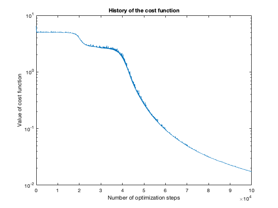
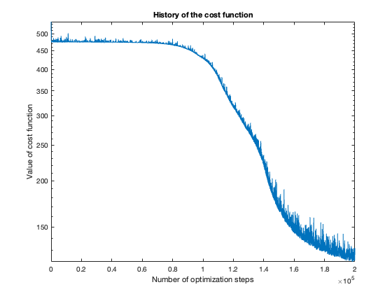
    semilogy(1:numbSteps,costHistory);
    xlabel('Number of optimization steps');
    ylabel('Value of cost function');
    title('History of the cost function')

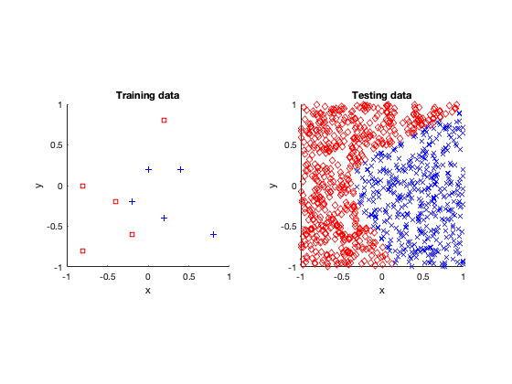
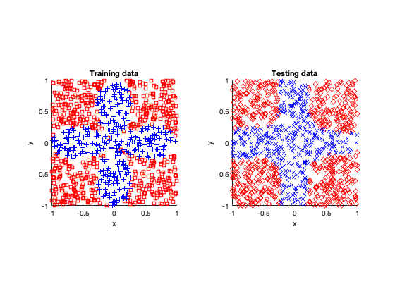
    %plot training data
    figure;
    tiledlayout(1,2);
    nexttile;
    hold on;
    plot(x1(booleTrain(1,:)),x2(booleTrain(1,:)),'rs');
    plot(x1(booleTrain(2,:)),x2(booleTrain(2,:)),'b+');
    xlabel('x');
    ylabel('y');
    title('Training data');
    axis([-1,1,-1,1]);
    axis square;

    %plot test data

    nexttile;
    hold on;
    plot(xTest1(booleTest(1,:)),xTest2(booleTest(1,:)),'rd');
    plot(xTest1(booleTest(2,:)),xTest2(booleTest(2,:)),'bx');
    xlabel('x');
    ylabel('y');
    title('Testing data');
    axis([-1,1,-1,1]);
    axis square;

end

function costTotal = getCost(x,y,arrayW,array_b,numbLayer)
numbTrainAll = max(size(x));
%originally y, x1 and x2 were defined outside this function
costAll = zeros(numbTrainAll,1);

for i = 1:numbTrainAll
    %loop through every training point
    x_i = x(:,i);

    A_Last=feedForward(x_i,arrayW,array_b,numbLayer);
    %find difference between algorithm output and training data
    costAll(i) = norm(y(:,i) - A_Last,2);
end
costTotal = norm(costAll,2)^2;
end

function y = activate(x,W,b)
z=(W*x+b);
%evaluate sigmoid (ie logistic) function
y = 1./(1+exp(-z));

%evaluate ReLU (rectified linear unit)
%y = max(0,z);
end

function A_Last= feedForward(xSingle,arrayW,array_b,numbLayer)
%run forward pass
A_now=xSingle;
for j=2:numbLayer
    A_next=activate(A_now,arrayW{j-1},array_b{j-1});
    A_now=A_next;
end


A_Last=A_next;
end

function booleFlowerInside=checkFlowerInside(x1,x2)
% This function creates a simple binary classification problem.
% A single point (x1,x2) is either inside a flower petal or not, where the
% flower (or rose) is defined in polar coordinates by the equation:
%
% rho(theta) =cos(k*theta)), where k is a positive integer.

orderFlower = 2;
[thetaFlower, rhoFlower] = cart2pol(x1(:)',x2(:)');
% check if point (x1,x2) is inside the rose
booleFlowerInside = abs(cos(orderFlower*thetaFlower)) <= rhoFlower;

end

function booleVoronoiInside=checkVoronoiInside(x1,x2)
% This function creates a simple binary classification problem.
% A single point (x1,x2) is either inside a chosen Voronoi cell or not,
% where the Voronoi cells are defined deterministically below.

numbPoints = length(x1);
% generat some deterministic seeds for the Voronoi cells
numbSeed = 6;
indexCellChosen = 4; %arbitrary chosen cells from first up to this number

t = 1:numbSeed;
% a deterministic points located on the square [-1,+1]x[-1,+1]
xSeed1 = sin(27*t.*pi.*cos(t.^2*pi+.4)+1.4);
xSeed2 = sin(4.7*t.*pi.*sin(t.^3*pi+.7)+.3);
xSeed = [xSeed1;xSeed2];

% find which Voroinoi cells each point (x1,x2) belongs to
indexVoronoi = zeros(1,numbPoints);
for i = 1:numbPoints
    x_i = [x1(i);x2(i)]; %retrieve single point
    diff_x = xSeed-x_i;
    distSquared_x = diff_x(1,:).^2+diff_x(2,:).^2; %relative distance squared
    [~,indexVoronoiTemp] = min(distSquared_x); %find closest seed
    indexVoronoi(i) = indexVoronoiTemp;
end

% see if points are inside the Voronoi cell number indexCellSingle
booleVoronoiInside = (indexVoronoi==indexCellChosen);
end

Python

The use of matrices in Python are kindly described as an afterthought. So it takes a bit of Python sleight of hand to get MATLAB code translated into working Python code.

(This stems partly from the fact that Python is row-major, as the language it’s built upon, C, whereas MATLAB is column-major, as its inspiration, Fortran.)

# This code runs a simple feedforward neural network.
#
# The neural network is a multi-layer perceptron designed for a simple
# binary classification. The classification is determining whether a
# two-dimensional (Cartesian) point is located inside some given region or
# not.
#
# For the simple binary examples used here, the code seems to work for
# sufficiently large number of optimization steps, typically in the 10s and
# 100s of thousands.
#
# This neural network only has 4 layers (so 2 hidden layers). The
# trainning procedure, meaning the forward and backward passes, are
# hard-coded. This means changing the number of layers requires additional
# information on the neural network architecture.
#
# It uses the sigmoid function; see the activate function.
#
# NOTE: This code is for illustration and educational purposes only. Use a
# industry-level library for real problems.
#
# For more details, see the post:
#
# https://hpaulkeeler.com/creating-a-simple-feedforward-neural-network-without-libraries/
#
# Author: H. Paul Keeler, 2019.
# Website: hpaulkeeler.com
# Repository: github.com/hpaulkeeler/posts

import numpy as np;  # NumPy package for arrays, random number generation, etc
import matplotlib.pyplot as plt  # For plotting
#from FunctionsExamples import checkFlowerInside, checkVoronoiInside

plt.close('all');  # close all figures

choiceData=1; #choose 1, 2 or 3

numbSteps = 1e5; #number of steps for the (gradient) optimization method
rateLearn = 0.05; #hyperparameter
numbTest = 1000; #number of points for testing the fitted model
boolePlot = True;

np.random.seed(42); #set seed for reproducibility of results

#helper functions for generating problems
def checkFlowerInside(x1,x2):
    # This function creates a simple binary classification problem.
    # A single point (x1,x2) is either inside a flower petal or not, where the
    # flower (or rose) is defined in polar coordinates by the equation:
    #
    # rho(theta) =cos(k*theta)), where k is a positive integer.

    orderFlower = 2;
    thetaFlower = np.arctan2(x2,x1);
    rhoFlower = np.sqrt(x1**2+x2**2);
    # check if point (x1,x2) is inside the rose
    booleFlowerInside = np.abs(np.cos(orderFlower*thetaFlower)) <= rhoFlower;
    return booleFlowerInside

def checkVoronoiInside(x1,x2):
    # This function creates a simple binary classification problem.
    # A single point (x1,x2) is either inside a chosen Voronoi cell or not,
    # where the Voronoi cells are defined deterministically below.
    numbPoints = len(x1);
    # generat some deterministic seeds for the Voronoi cells
    numbSeed = 6;
    indexCellChosen = 4; #arbitrary chosen cells from first up to this number

    t = np.arange(numbSeed)+1;
    # a deterministic points located on the square [-1,+1]x[-1,+1]
    xSeed1 = np.sin(27*t*np.pi*np.cos(t**2*np.pi+.4)+1.4);
    xSeed2 = np.sin(4.7*t*np.pi*np.sin(t**3*np.pi+.7)+.3);
    xSeed = np.stack((xSeed1,xSeed2),axis=0);

    # find which Voroinoi cells each point (x1,x2) belongs to
    indexVoronoi = np.zeros(numbPoints);
    for i in range(numbPoints):
        x_i = np.stack((x1[i],x2[i]),axis=0).reshape(-1, 1); #retrieve single point
        diff_x = xSeed-x_i;
        distSquared_x = diff_x[0,:]**2+diff_x[1,:]**2; #relative distance squared
        indexVoronoiTemp = np.argmin(distSquared_x); #find closest seed
        indexVoronoi[i] = indexVoronoiTemp;

    # see if points are inside the Voronoi cell number indexCellSingle
    booleVoronoiInside = (indexVoronoi==indexCellChosen);
    return booleVoronoiInside


#generating or retrieving the training data
if (choiceData==1):
    ### simple example
    #recommended minimum number of optimization steps: numbSteps = 1e5
    x1 = 2*np.array([0.1,0.3,0.1,0.6,0.4,0.6,0.5,0.9,0.4,0.7])-1;
    x2 = 2*np.array([0.1,0.4,0.5,0.9,0.2,0.3,0.6,0.2,0.4,0.6])-1;
    numbTrainAll = 10; #number of training data
    #output (binary) data
    y = np.array([[1,1,1,1,1,0,0,0,0,0],[0,0,0,0,0,1,1,1,1,1]]);

    x=np.stack((x1,x2),axis=0);

if (choiceData==2):
    ### voronoi example
    #recommended minimum number of optimization steps: numbSteps = 1e5
    numbTrainAll = 500; #number of training data
    x=2*np.random.uniform(0, 1,(2,numbTrainAll))-1;
    x1 = x[0,:];
    x2 = x[1,:];
    booleInsideVoroni=checkVoronoiInside(x1,x2);
    # output (binary) data
    y=np.stack((booleInsideVoroni,~booleInsideVoroni),axis=0);

if (choiceData==3):
    ### rose/flower example
    #recommended minimum number of optimization steps: numbSteps = 2e5
    numbTrainAll=100; #number of training data
    x=2*np.random.uniform(0, 1,(2,numbTrainAll))-1;
    x1 = x[0,:];
    x2 = x[1,:];
    booleInsideFlower=checkFlowerInside(x1,x2);
    #output (binary) data
    y=np.stack((booleInsideFlower,~booleInsideFlower),axis=0);

#helper functions for training and running the neural network
def activate(x,W,b):
    z=np.matmul(W,x)+b;
    #evaluate sigmoid (ie logistic) function
    y = 1/(1+np.exp(-z));

    #evaluate ReLU (rectified linear unit)
    #y = np.max(0,z);
    return y

def feedForward(xSingle,arrayW,array_b,numbLayer):
    #run forward pass
    A_now=xSingle;
    for j in np.arange(1,numbLayer):
        A_next=activate(A_now,arrayW[j-1],array_b[j-1]);
        A_now=A_next;
    A_Last=A_next;

    return A_Last;


def getCost(x,y,arrayW,array_b,numbLayer):
    numbTrainAll = np.max(x.shape);
    #originally y, x1 and x2 were defined outside this function
    costAll = np.zeros((numbTrainAll,1));

    for i in range(numbTrainAll):
        #loop through every training point
        x_i = x[:,i].reshape(-1, 1);

        A_Last=feedForward(x_i,arrayW,array_b,numbLayer);
        #find difference between algorithm output and training data
        costAll[i] = np.linalg.norm(y[:,i].reshape(-1, 1) - A_Last,2);

        costTotal = np.linalg.norm(costAll,2)**2;

    return costTotal

#dimensions/widths of neural network
numbWidth1 = 2; #must be 2 for 2-D input data
numbWidth2 = 4;
numbWidth3 = 4;
numbWidth4 = 2; #must be 2 for binary output
numbWidthAll=np.array([numbWidth1,numbWidth2,numbWidth3,numbWidth4]);
numbLayer=len(numbWidthAll);

#initialize weights and biases
scaleModel = .5;
W2 = scaleModel * np.random.normal(0, 1,(numbWidth2,numbWidth1));
b2 = scaleModel * np.random.uniform(0, 1,(numbWidth2,1));
W3 = scaleModel * np.random.normal(0, 1,(numbWidth3,numbWidth2));
b3 = scaleModel * np.random.uniform(0, 1,(numbWidth3,1));
W4 = scaleModel * np.random.normal(0, 1,(numbWidth4,numbWidth3));
b4 = scaleModel * np.random.uniform(0, 1,(numbWidth4,1));

#create lists of matrices
#w matrices
arrayW=[];
arrayW.append(W2);
arrayW.append(W3);
arrayW.append(W4);
#b vectors
array_b=[];
array_b.append(b2);
array_b.append(b3);
array_b.append(b4);
#activation matrices
arrayA=[];
for j in range(numbLayer):
    arrayA.append(np.zeros(numbWidthAll[j]).reshape(-1, 1).T);
#delta (gradient) vectors
array_delta=[];
for j in range(numbLayer-1):
    array_delta.append(np.zeros(numbWidthAll[j+1]).reshape(-1, 1).T);

numbSteps=int(numbSteps)
costHistory = np.zeros((numbSteps,1));
booleTrain = y;
for i in range(numbSteps):
    #forward and back propagation
    indexTrain=np.random.randint(numbTrainAll);
    xTrain = x[:,indexTrain].reshape(-1, 1);

    #run forward pass
    arrayA[0]=xTrain; #treat input as the A1 matrix
    for j in (range(numbLayer-1)):
        arrayA[j+1]=activate(arrayA[j],arrayW[j],array_b[j]);

    #run backward pass (to calculate the gradient) using Hadamard products
    A_temp=arrayA[-1];
    array_delta[-1]=A_temp*(1-A_temp)*(A_temp-y[:,indexTrain].reshape(-1, 1));
    for j in np.arange(numbLayer-2,0,-1):
        A_temp=arrayA[j];
        delta_temp=array_delta[j];
        W_temp=arrayW[j];
        array_delta[j-1]= A_temp*(1-A_temp)*np.matmul(np.transpose(W_temp),delta_temp);


    #update using steepest descent
    #transpose of xTrains used for W matrices
    for j in range(numbLayer-1):
        A_temp=arrayA[j];
        delta_temp=array_delta[j];
        arrayW[j]=arrayW[j] - rateLearn*np.matmul(delta_temp,np.transpose(A_temp));
        array_b[j]=array_b[j] - rateLearn*delta_temp;


    #update cost
    costCurrent_i = getCost(x,y,arrayW,array_b,numbLayer);
    costHistory[i] = costCurrent_i;

#generating test data
xTest = 2*np.random.uniform(0,1,(2,numbTest))-1;
xTest1 = xTest[0,:];
xTest2 = xTest[1,:];

booleTest = np.zeros((2,numbTest));

#testing every point
for k in range(numbTest):
    xTestSingle = xTest[:,k].reshape(-1, 1);
    #apply fitted model
    yTestSingle = feedForward(xTestSingle,arrayW,array_b,numbLayer);
    indexTest = np.argmax(yTestSingle, axis=0);
    booleTest[0,k] = ((indexTest==0)[0]);
    booleTest[1,k] = ((indexTest==1)[0]);

if boolePlot:
    #plot history of cost
    plt.figure();
    plt.semilogy(np.arange(numbSteps)+1,costHistory);
    plt.xlabel('Number of optimization steps');
    plt.ylabel('Value of cost function');
    plt.title('History of the cost function')

    #plot training data
    fig, ax = plt.subplots(1, 2);
    ax[0].plot(x1[np.where(booleTrain[0,:])],x2[np.where(booleTrain[0,:])],\
        'rs', markerfacecolor='none');
    ax[0].plot(x1[np.where(booleTrain[1,:])],x2[np.where(booleTrain[1,:])],\
        'b+');
    ax[0].set_xlabel('x');
    ax[0].set_ylabel('y');
    ax[0].set_title('Training data');
    ax[0].set_xlim([-1, 1])
    ax[0].set_ylim([-1, 1])
    ax[0].axis('equal');

    #plot test data
    ax[1].plot(xTest1[np.where(booleTest[0,:])],xTest2[np.where(booleTest[0,:])],\
        'rd', markerfacecolor='none');
    ax[1].plot(xTest1[np.where(booleTest[1,:])],xTest2[np.where(booleTest[1,:])],\
        'bx');
    ax[1].set_xlabel('x');
    ax[1].set_ylabel('y');
    ax[1].set_title('Testing data');
    ax[1].set_xlim([-1, 1])
    ax[1].set_ylim([-1, 1])
    ax[1].axis('equal');

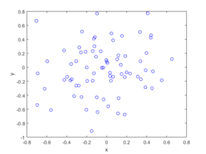
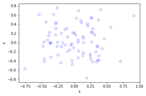
Results

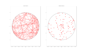
After fitting or training the models, I tested them by applying the fitted neural network to other data. (In machine learning and statistics, you famously don’t use the same data to train and test a model.)

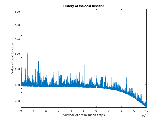
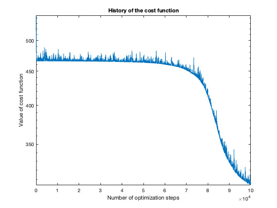
The number of steps needed to obtain reasonable results was about 100 thousand. To get a feeling of this, look at the plot of the cost function value over the number of optimization steps. For more complicated problems, such as the flower or rose problem, even more steps were needed.

I found the Python code, which is basically a close literal translation (by me) of the MATLAB code, too slow, so I generated the results using MATLAB.

Note: These results were generated with stochastic methods (namely, the training method), so my results will not agree exactly with yours, but hopefully they’ll be close enough.

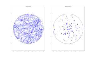
Simple

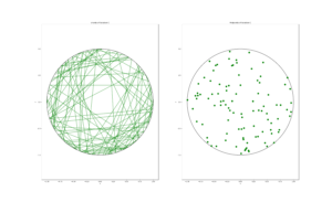
Voronoi

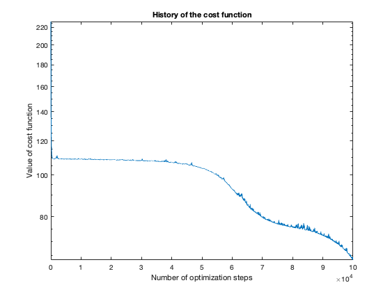
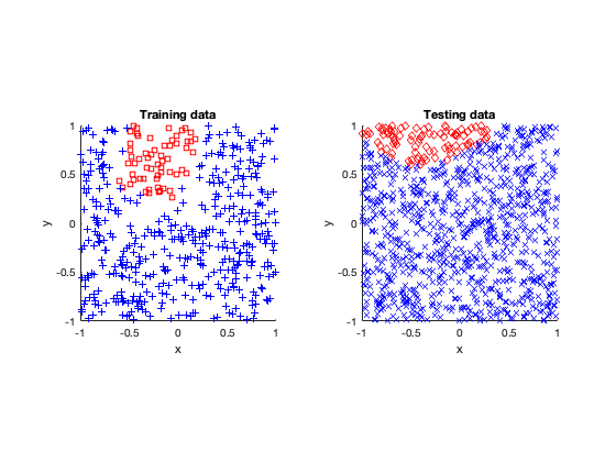
Rose

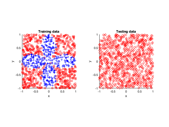
The rose problem was the most difficult to classify. Sometimes it was a complete fail. Sometimes the training method could only see one component of the rose. It worked a couple of times, namely with 20 thousand optimization steps and a random seed of 42.

I imagine this problem is difficult due to the obvious complex geometry. Specifically, the both ends of each petal become thin, which is where the testing breaks down.

Fail

Half-success

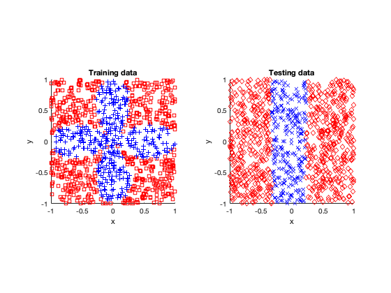
Success (mostly)

The Bertrand paradox

Mathematical paradoxes are results or observations in mathematics that are (seemingly) conflicting, unintuitive, incomprehensible, or just plain bizarre. They come in different flavours, such as those that play with notions of infinity, which means they often make little or no sense in a physical world. Other paradoxes, particularly those in probability, serve as a lesson that the problem needs to be posed in a precise manner. The Bertrand paradox is one of these.

Joseph Bertrand posed the original problem in his 1889 book Calcul des probabilités, which is available online (in French); page 4, Section 5. It’s a great illustrative problem involving simple probability and geometry, so it often appears in literature on the (closely related) mathematical fields of geometric probability and integral geometry.

Based on constructing a random chord in a circle, Bertrand’s paradox involves a single mathematical problem with three reasonable but different solutions. It’s less a paradox and more a cautionary tale. It’s really asking the question: What exactly do you mean by random?

Consequently, over the years the Bertrand paradox has inspired debate, with papers arguing what the true solution is. I recently discovered it has even inspired some passionate remarks on the internet; read the comments at www.bertrands-paradox.com.

Update: The people from Numberphile and 3Blue1Brown have recently produced a video on YouTube describing and explaining the Bertrand paradox.

But I am less interested in the different interpretations or philosophies of the problem. Rather, I want to simulate the three solutions. This is not very difficult, provided some trigonometry and knowledge from a previous post, where I describe how to simulate a (homogeneous) Poisson point process on the disk.

I won’t try to give a thorough analysis of the solutions, as there are much better websites doing that. For example, this MIT website gives a colourful explanation with pizza and fire-breathing monsters. The Wikipedia article also gives a detailed though less creative explanation for the three solutions.

My final code in MATLAB, R and Python code is located here.

The Problem

Bertrand considered a circle with an equilateral triangle inscribed it. If a chord in the circle is randomly chosen, what is the probability that the chord is longer than a side of the equilateral triangle?

The Solution(s)

Bertrand argued that there are three natural but different methods to randomly choose a chord, giving three distinct answers. (Of course, there are other methods, but these are arguably not the natural ones that first come to mind.)

Method 1: Random endpoints

On the circumference of the circle two points are randomly (that is, uniformly and independently) chosen, which are then used as the two endpoints of the chord.

The probability of this random chord being longer than a side of the triangle is one third.

Method 2: Random radius

A radius of the circle is randomly chosen (so the angle is chosen uniformly), then a point is randomly (also uniformly) chosen along the radius, and then a chord is constructed at this point so it is perpendicular to the radius.

The probability of this random chord being longer than a side of the triangle is one half.

Method 3: Random midpoint

A point is randomly (so uniformly) chosen in the circle, which is used as the midpoint of the chord, and the chord is randomly (also uniformly) rotated.

The probability of this random chord being longer than a side of the triangle is one quarter.

Simulation

All three answers involve randomly and independently sampling two random variables, and then doing some simple trigonometry. The setting naturally inspires the use of polar coordinates. I assume the circle has a radius $r$ and a centre at the origin $o$. I’ll arbitrarily number the end points one and two.

In all three solutions we need to generate uniform random variables on the interval $(0, 2\pi)$ to simulate random angles. I have already done this a couple of times in previous posts such as this one.

Method 1: Random endpoints

This is probably the most straightforward solution to simulate. We just need to simulate two uniform random variables $\Theta_1$ and $\Theta_2$ on the interval $(0, 2\pi)$ to describe the angles of the two points.

The end points of the chord (in Cartesian coordinates) are then simply:

Point 1: $X_1=r \cos \Theta_1$, $Y_1=r \sin \Theta_1$,

Point 2: $X_2=r \cos \Theta_2$, $Y_2=r \sin \Theta_2$.

Method 2: Random radius

This method also involves generating two uniform random variables. One random variable $\Theta$ is for the angle, while the other $P$ is the random radius, which means generating the random variable $P$ on the interval $(0, r)$.

I won’t go into the trigonometry, but the random radius and its perpendicular chord create a right-angle triangle. The distance from the point $(\Theta, P)$ to the circle along the chord is:

$$Q=\sqrt{r^2-P^2}.$$

The endpoints of the chord are then:

Point 1: $X_1=P \cos \Theta+ Q\sin \Theta$, $Y_1= P \sin \Theta- Q\cos \Theta$,

Point 2: $X_2=P \cos \Theta- Q\sin \Theta$, $Y_2= P \sin \Theta+Q \cos \Theta$.

Take note of the signs in these expressions.

Method 3: Random midpoint

This method requires placing a point uniformly on a disk, which is also done when simulating a homogeneous Poisson point process on a disk, and requires two random variables $\Theta’$ and $P’$. Again, the angular random variable $\Theta’$ is uniform.

The other random variable $P’$ is not uniform. For $P’$, we generate a random uniform variable on the unit interval $(0,1)$, and then we take the square root of it. We then multiply it by the radius, generating a random variable between $0$ and $r$. (We must take the square root because the area element of a sector is proportional to the radius squared, and not the radius.) The distribution of this random variable is an example of the triangular distribution.

The same trigonometry from Method 2 applies here, which gives the endpoints of the chord as:

Point 1: $X_1=P’ \cos \Theta’+ Q’\sin \Theta’$, $Y_1= P’ \sin \Theta’- Q’\cos \Theta’$,

Point 2: $X_2=P’\cos \Theta’- Q’\sin \Theta’$, $Y_2= P’\sin \Theta’+Q’ \cos \Theta’$,

where $Q’:=\sqrt{r^2-{P’}^2}$. Again, take note of the signs in these expressions.

Results

To illustrate how the three solutions are different, I’ve plotted a hundred random line segments and their midpoints side by side. Similar plots are in the Wikipedia article.

Method 1: Random endpoints

Method 2: Random radius

Method 3: Random midpoint

Conclusion

For the chord midpoints, we know and can see that Method 3 gives uniform points, while Method 2 has a concentration of midpoints around the circle centre. Method 1 gives results that seem to somewhere between Method 2 and 3 in terms of clustering around the circle centre.

For the chords, we see that Method 3 results in fewer chords passing through the circle centre. Methods 1 and 2 seem to give a similar number of lines passing through this central region.

It’s perhaps hard to see, but it can be shown that Method 2 gives the most uniform results. By this, I mean that the number of lines and their orientations statistically do not vary in different regions of the circle.

We can now position random lines in uniform manner. All we need now is a Poisson number of lines to generate something known as a Poisson line process, which will be the subject of the next post.

Code

The MATLAB, R and Python code can be found here. In the code, I have labelled the methods A, B and C instead 1, 2 and 3.

Testing the Julia language with point process simulations

I started writing these posts (or blog entries) about a year ago. In my first post I remarked how I wanted to learn to write stochastic simulations in a new language. Well, I found one. It’s called Julia. Here’s my code. And here are my thoughts.

Overview

For scientific programming, the Julia language has arisen as a new contender. Originally started in 2012, its founders and developers have (very) high aspirations, wanting the language to be powerful and accessible, while still having run speeds comparable to C. There’s been excitement about it, and even a Nobel Laureate in economics, Thomas Sargent, has endorsed it. He co-founded the QuantEcon project, whose website has this handy guide or cheat sheet for commands between MATLAB, Python and Julia.

That guide suggests that Julia’s main syntax inspiration comes from MATLAB. But perhaps its closest (and greatest) competitor in scientific programming languages is Python, which has become a standard language used in scientific programming, particularly in machine learning. Another competitor is the statistics language R, which is popular for data science. But R is not renown for its speed.

As an aside, machine learning is closely related to what many call data science. I consider the two disciplines as largely overlapping with statistics, where their respective emphases are on theory and practice. In these fields, often the languages Python and R are used. There are various websites discussing which language is better, such as this one, which in turn is based on this one. In general, it appears that computer scientists and statisticians respectively prefer using Python and R.

Returning to the Julia language, given its young age, the language is still very much evolving, but I managed to find suitable Julia functions for stochastic simulations. I thought I would try it out by simulating some point processes, which I have done several times before. I successfully ran all my code with Julia Version 1.0.3.

In short, I managed to replicate in (or even translate to) Julia the code that I presented in the following posts:

Simulating a homogeneous Poisson point process on a rectangle

Simulating a Poisson point process on a disk

Simulating a Poisson point process on a triangle

Simulating an inhomogeneous Poisson point process

Simulating a Matérn cluster point process

Simulating a Thomas cluster point process

The Julia code, like all the code I present here, can be found on my Github repository, which for this post is located here.

Basics

Language type and syntax

The Wikipedia article on Julia says:

Julia is a high-level general-purpose dynamic programming language designed for high-performance numerical analysis and computational science.

Scientific programming languages like the popular three MATLAB, R and Python, are interpreted languages. But the people behind Julia say:

it is a flexible dynamic language, appropriate for scientific and numerical computing, with performance comparable to traditional statically-typed languages.

Because Julia’s compiler is different from the interpreters used for languages like Python or R, you may find that Julia’s performance is unintuitive at first.

I already remarked that Julia’s syntax is clearly inspired by MATLAB, as one can see in this guide for MATLAB, Python and Julia. But there are key differences. For example, to access an array entry in Julia, you use square brackets (like in most programming languages), whereas parentheses are used in MATLAB or, that old mathematical programming classic, Fortran, which is not a coincidence.

Packages

Julia requires you to install certain packages or libraries, like most languages. For random simulations and plots, you have to install the respective Julia packages Distributions and Plots, which is done by running the code.

Pkg.add("Distributions");
Pkg.add("Plots");

After doing that, it’s best to restart Julia. These packages are loaded with the using command:

Using Distributions;
Using Plots;

Also, the first time it takes a while to run any code using those newly installed packages.

I should stress that there are different plotting libraries. But Plots, which contains many plotting libraries, is the only one I could get working. Another is PlotPy, which uses the Python library. As a beginner, it seems to me that the Julia community has not focused too much on developing new plotting functions, and has instead leveraged pre-existing libraries.

For standard scientific and statistical programming, you will usually also need the packages LinearAlgebra and Statistics.

Data types

Unlike MATLAB or R, Julia is a language that has different data types for numbers, such as integers and floating-point numbers (or floats). This puts Julia in agreement with the clear majority of languages, making it nothing new for most programmers. This is not a criticism of the language, but this can be troublesome if you’ve grown lazy after years of using MATLAB and R.

Simulating random variables

In MATLAB, R and Python, we just need to call a function for simulating uniform, Poisson, and other random variables. There’s usually a function for each type of random variable (or probability distribution).

Julia does simulation of random objects in a more, let’s say, object-oriented way (but I’m told, it’s not an object-oriented language). The probability distributions of random variables are objects, which are created and then sent to a general function for random generation. For example, here’s the code for simulating a Poisson variable with mean $\mu=10$.

mu=10;
distPoisson=Poisson(mu);
numbPoisson=rand(distPoisson);

Similarly, here’s how to simulate a normal variable with mean $\mu=10$ and standard deviation $\sigma=1$.

mu=10;
sigma=1;
distNormal=Normal(mu,sigma);
numbNormal=rand(distNormal);

Of course the last two lines can be collapsed into one.

mu=10;
sigma=1;
numbNormal=rand(Normal(mu,sigma));

But if you just want to create standard uniform variables on the interval (0,1), then the code is like that in MATLAB. For example, this code creates a $4\times3$ matrix (or array) $X$ whose entries are simulation outcomes of independent uniform random variables:

X=rand(4,3);

The resulting matrix $X$ is a Float 64 array.

Arrays

The indexing of arrays in Julia starts at one, just like MATLAB, R, or Fortran. When you apply a function to an array, you generally need to use the dot notation. For example, if I try to run the code:

Y=sqrt(rand(10,1)); #This line will result in an error.

then on my machine (with Julia Version 1.0.3) I get the error:

ERROR: DimensionMismatch(“matrix is not square: dimensions are (10, 1)”)

But this code works:

Y=sqrt.(rand(10,1));

Also, adding scalars to arrays can catch you in Julia, as you also often need to use the dot notation. This code:

Y=sqrt.(rand(10,1));
Z=Y+1; #This line will result in an error.

gives the error:

ERROR: MethodError: no method matching +(::Array{Float64,2}, ::Int64)

This is fixed by adding a dot:

Y=sqrt.(rand(10,1));
Z=Y.+1; #This line will work.

Note the dot has to be on the left hand side. I ended up just using dot notation every time to be safe.

Other traps exist. For example, with indexing, you need to convert floats to integers if you want to use them as indices.

Repeating array elements

There used to be a Julia function called repmat, like the one in MATLAB , but it was merged with a function called repeat. I used such repeating operations to avoid explicit for-loops, which is generally advised in languages like MATLAB and R. For example, I used the repelem function in MATLAB to simulate Matérn and Thomas cluster point processes. To do this in Julia, I had to use this nested construction:

y=vcat(fill.(x, n)...);

This line means that the first value in $x $ is repeated $n[1]$ times, where $n[1]$ is the first entry of $n$ (as indexing in Julia starts at one), then the second value of $x$ is repeated $n[2]$ times, and so on. For example, the vectors $x=[7,4,9]$ and $n=[2,1,3]$, the answer is $y=[7,7,4,9,9,9]$.

To do this in Julia, the construction is not so bad, if you know how, but it’s not entirely obvious. In MATLAB I use this:

y=repelem(x,n);

Similarly in Python:

y=np.repeat(x,n);

Different versions of Julia

I found that certain code would work (or not work) and then later the same code would not work (or would work) on machines with different versions of Julia, demonstrating how the language is still being developed. More specifically, I ran code on Julia Version 1.0.3 (Date 2018-12-18) and Julia Version 0.6.4 (Date: 2018-07-09). (Note how there’s only a few months difference in the dates of the two versions.)

Consider the code with the errors (due to the lack of dot operator) in the previous section. The errors occurred on one machine with Julia Version 1.0.3, but the errors didn’t occur on another machine with the older Julia Version 0.6.4. For a specific example, the code:

Y=sqrt.(rand(10,1));
Z=Y+1; #This line will not result in an error on Version 0.6.4.

gives no error with Julia Version 0.6.4, while I have already discussed how it gives an error with Julia Version 1.0.3.

For another example, I copied from this MATLAB-Python-Julia guide the following command:

A = Diagonal([1,2,3]); #This line will (sometimes?) result in an error.

It runs on machine with Julia Version 0.6.4 with no problems. But running it on the machine with Julia Version 1.0.3 gives the error:

ERROR: UndefVarError: Diagonal not defined

That’s because I have not used the LinearAlgebra package. Fixing this, the following code:

using LinearAlgebra; #Package needed for Diagonal command.
A = Diagonal([1,2,3]); #This line should now work.

gives no error with Julia Version 1.0.3.

If you have the time and energy, you can search the internet and find online forums where the Julia developers have discussed why they have changed something, rendering certain code unworkable with the latest versions of Julia.

Optimization

It seems that performing optimization on functions is done with the Optim package.

Pkg.add("Optim");

But some functions need the Linesearches package, so it’s best to install that as well.

Pkg.add("Linesearches");

Despite those two optimization packages, I ended up using yet another package called BlackBoxOptim.

Pkg.add("BlackBoxOptim");

In this package, I used a function called bboptimize. This is the first optimziation function that I managed to get working. I do not know how it compares to the functions in the Optim and Linesearches packages.

In a previous post, I used optimization functions to simulate a inhomogeneous or nonhomogeneous Poisson point process on a rectangle. I’ve also written Julia code for this simulation, which is found below. I used bboptimize, but I had some problems when I initially set the search regions to integers, which the package did not like, as the values need to be floats. That’s why I multiple the rectangle dimensions by $1.0$ in the following code:

boundSearch=[(1.0xMin,1.0xMax), (1.0yMin, 1.0yMax)]; #bounds for search box
#WARNING: Values of boundSearch cannot be integers!
resultsOpt=bboptimize(fun_Neg;SearchRange = boundSearch);
lambdaNegMin=best_fitness(resultsOpt); #retrieve minimum value found by bboptimize

Conclusion

In this brief experiment, I found the language Julia good for doing stochastic simulations, but too tricky for doing simple things like plotting. Also, depending on the version of Julia, sometimes my code would work and sometimes it wouldn’t. No doubt things will get better with time.

Code

I’ve only posted here code for some of simulations, but the rest of the code is available on my GitHub repository located here. You can see how the code is comparable to that of MATLAB.

Poisson point process on a rectangle

I wrote about this point process here. The code is located here.

using Distributions #for random simulations
using Plots #for plotting

#Simulation window parameters
xMin=0;xMax=1;
yMin=0;yMax=1;
xDelta=xMax-xMin;yDelta=yMax-yMin; #rectangle dimensions
areaTotal=xDelta*yDelta;

#Point process parameters
lambda=100; #intensity (ie mean density) of the Poisson process

#Simulate Poisson point process
numbPoints=rand(Poisson(areaTotal*lambda)); #Poisson number of points
xx=xDelta*rand(numbPoints,1).+xMin;#x coordinates of Poisson points
yy=yDelta*(rand(numbPoints,1)).+yMin;#y coordinates of Poisson points

#Plotting
plot1=scatter(xx,yy,xlabel ="x",ylabel ="y", leg=false);
display(plot1);

Inhomogeneous Poisson point process on a rectangle

I wrote about this point process here. The code is located here.

using Distributions #for random simulations
using Plots #for plotting
using BlackBoxOptim #for blackbox optimizing

#Simulation window parameters
xMin=-1;xMax=1;
yMin=-1;yMax=1;
xDelta=xMax-xMin;yDelta=yMax-yMin; #rectangle dimensions
areaTotal=xDelta*yDelta;

s=0.5; #scale parameter

#Point process parameters
function fun_lambda(x,y)
    100*exp.(-(x.^2+y.^2)/s^2); #intensity function
end

###START -- find maximum lambda -- START ###
#For an intensity function lambda, given by function fun_lambda,
#finds the maximum of lambda in a rectangular region given by
#[xMin,xMax,yMin,yMax].
#NOTE: Need xMin, xMax, yMin, yMax to be floats eg xMax=1. See boundSearch

function fun_Neg(x)
     -fun_lambda(x[1],x[2]); #negative of lambda
end
xy0=[(xMin+xMax)/2.0,(yMin+yMax)/2.0];#initial value(ie centre)

#Find largest lambda value
boundSearch=[(1.0xMin,1.0xMax), (1.0yMin, 1.0yMax)];
#WARNING: Values of boundSearch cannot be integers!
resultsOpt=bboptimize(fun_Neg;SearchRange = boundSearch);
lambdaNegMin=best_fitness(resultsOpt); #retrieve minimum value found by bboptimize
lambdaMax=-lambdaNegMin;
###END -- find maximum lambda -- END ###

#define thinning probability function
function fun_p(x,y)
    fun_lambda(x,y)/lambdaMax;
end

#Simulate a Poisson point process
numbPoints=rand(Poisson(areaTotal*lambdaMax)); #Poisson number of points
xx=xDelta*rand(numbPoints,1).+xMin;#x coordinates of Poisson points
yy=yDelta*(rand(numbPoints,1)).+yMin;#y coordinates of Poisson points

#calculate spatially-dependent thinning probabilities
p=fun_p(xx,yy);
#Generate Bernoulli variables (ie coin flips) for thinning
booleRetained=rand(numbPoints,1).<p; #points to be retained
xxRetained=xx[booleRetained]; yyRetained=yy[booleRetained];

#Plotting
plot1=scatter(xxRetained,yyRetained,xlabel ="x",ylabel ="y", leg=false);
display(plot1);

Thomas point process on a rectangle

I wrote about this point process here. The code is located here.

using Distributions #for random simulations
using Plots #for plotting

#Simulation window parameters
xMin=-.5;
xMax=.5;
yMin=-.5;
yMax=.5;

#Parameters for the parent and daughter point processes
lambdaParent=10;#density of parent Poisson point process
lambdaDaughter=10;#mean number of points in each cluster
sigma=0.05; #sigma for normal variables (ie random locations) of daughters

#Extended simulation windows parameters
rExt=7*sigma; #extension parameter
#for rExt, use factor of deviation sigma eg 6 or 7
xMinExt=xMin-rExt;
xMaxExt=xMax+rExt;
yMinExt=yMin-rExt;
yMaxExt=yMax+rExt;
#rectangle dimensions
xDeltaExt=xMaxExt-xMinExt;
yDeltaExt=yMaxExt-yMinExt;
areaTotalExt=xDeltaExt*yDeltaExt; #area of extended rectangle

#Simulate Poisson point process
numbPointsParent=rand(Poisson(areaTotalExt*lambdaParent)); #Poisson number of points

#x and y coordinates of Poisson points for the parent
xxParent=xMinExt.+xDeltaExt*rand(numbPointsParent,1);
yyParent=yMinExt.+yDeltaExt*rand(numbPointsParent,1);

#Simulate Poisson point process for the daughters (ie final poiint process)
numbPointsDaughter=rand(Poisson(lambdaDaughter),numbPointsParent);
numbPoints=sum(numbPointsDaughter); #total number of points

#Generate the (relative) locations in Cartesian coordinates by
#simulating independent normal variables
xx0=rand(Normal(0,sigma),numbPoints);
yy0=rand(Normal(0,sigma),numbPoints);

#replicate parent points (ie centres of disks/clusters)
xx=vcat(fill.(xxParent, numbPointsDaughter)...);
yy=vcat(fill.(yyParent, numbPointsDaughter)...);

#Shift centre of disk to (xx0,yy0)
xx=xx.+xx0;
yy=yy.+yy0;

#thin points if outside the simulation window
booleInside=((xx.>=xMin).&(xx.<=xMax).&(yy.>=yMin).&(yy.<=yMax));
#retain points inside simulation window
xx=xx[booleInside];
yy=yy[booleInside];

#Plotting
plot1=scatter(xx,yy,xlabel ="x",ylabel ="y", leg=false);
display(plot1);

Checking Poisson point process simulations

In previous posts I described how to simulate homogeneous Poisson point processes on a rectangle, disk and triangle. Then I covered how to randomly thin a point process in a spatially dependent manner. Building off these posts, I wrote in my last post how to simulate an inhomogeneous or nonhomogeneous Poisson point process. Now I’ll describe how to verify that the simulation code correctly simulates the desired Poisson point process.

Although this post is focused on the Poisson point process, I stress that parts of the material hold for all point processes. Also, not surprisingly, some of the material and the code overlaps with that presented in the post on the inhomogeneous point process.

Basics

Any Poisson point process is defined with a measure called the intensity measure or mean measure, which I’ll denote by $\Lambda$. For practical purposes, I assume that the intensity measure $\Lambda$ has a derivative $\lambda(x,y)$, where $x$ and $y$ denote the Cartesian coordinates. The function $\lambda(x,y)$ is often called the intensity function or just intensity. I assume this function is bounded, so $\lambda(x,y)<\infty$ for all points in a simulation window $W$. Finally, I assume that the simulation window $W$ is a rectangle.

Several times before I have mentioned that simulating a Poisson point process requires simulating two random components: the number of points and the locations of points. Working backwards, to check a Poisson simulation, we must run the Poisson simulation a large number of times (say $10^3$ or $10^4$), and collect the statistics on these two properties. We’ll start by examining the easiest of the two random components.

Number of points

For any Poisson point process, the number of points is a Poisson random variable with a parameter (that is, a mean) $\Lambda(W)$. Under our previous assumptions, this is given by the surface integral

$$\Lambda(W)=\int_W \lambda(x,y)dxdy.$$

Presumably we can evaluate such an integral analytically or numerically in order to simulate the Poisson point process. To check that we correctly simulate the random the number of points, we just need to simulate the point process a large number of times, and compare the statistics to those given by the analytic expressions.

Moments

The definition of the intensity measure of a point process is a measure that gives the average or expected number of points in some region. As the number of simulations increases, the (sample) average number of points will converge to the intensity measure $\Lambda(W)$. I should stress that this is a test for the intensity measure, a type of first moment, which will work for the intensity measure of any point process.

For Poisson point processes, there is another moment test that can be done. It can be shown mathematically that the variance of the number of points will also converge to the intensity measure $\Lambda(W)$, giving a second empirical test based on second moments. There is no point process theory here, as this moment result is simply due to the number of points being distributed according to a Poisson distribution. The second moment is very good for checking Poissonness, forming the basis for statistical tests. If this and the first moment test hold, then there’s a very strong chance the number of points is a Poisson variable.

Empirical distribution

Beyond the first two moments, an even more thorough test is to estimate an empirical distribution for the number of points. That is, we perform a histogram on the number of points, and then we normalize it, so the total mass sums to one, producing an empirical probability distribution for the number of points.

The results should closely match the probability mass function of a Poisson distribution with parameter $\Lambda(W)$. This is simply

$$ P(N=n)= \frac{[\Lambda(W)]^n}{n!} e^{-\Lambda(W)}, $$

where $N$ is the random number of points in the window $W$, which has the area $|W|$. If the empirical distribution is close to results given by the above expression, then we can confidently say that the number of points is a Poisson random variable with the right parameter or mean.

Locations of points

To check the positioning of points, we can empirically estimate the intensity function $\lambda(x,y)$. A simple way to do this is to perform a two-dimensional histogram on the point locations. This is very similar to the one-dimensional histogram, which I suggested to do for testing the number of points. It just involves counting the number of points that fall into two-dimensional non-overlapping subsets called bins.

To estimate the intensity function, each bin count needs to be rescaled by the area of the bin, giving a density value for each bin. This empirical estimate of the intensity function should resemble the true intensity function $\lambda(x,y)$. For a visual comparison, we can use a surface plot to illustrate the two sets of results.

This procedure will work for estimating the intensity function of any point process, not just a Poisson one.

Advanced tests

In spatial statistics there are more advanced statistical tests for testing how Poisson a point pattern is. But these tests are arguably too complicated for checking a simple point process that is rather easy to simulate. Furthermore, researchers usually apply these tests to a small number of point patterns. In this setting, it is not possible to accurately obtain empirical distributions without further assumptions. But with simulations, we can generate many simulations and obtain good empirical distributions. In short, I would not use such tests for just checking that I have properly coded a Poisson simulation.

Results

I produced the results with ten thousand simulations, which gave good results and took only a few seconds to complete on a standard desktop computer. Clearly increasing the number of simulations increases the accuracy of the statistics, but it also increases the computation time.

For the results, I used the intensity function

$$\lambda(x,y)=\lambda_1(x,y)+\lambda_2(x,y),$$

where

$$\lambda_1(x,y)=80e^{-((x+0.5)^2+(y+0.5)^2)/s^2},$$

$$\lambda_2(x,y)=100e^{-((x-0.5)^2+(y-0.5)^2)/s^2},$$

and $s>0$ is a scale parameter. We can see that this function has two maxima or peaks at $(-0.5,-0.5)$ and $(0.5,0.5)$.

MATLAB

Python

Code

All code from my posts, as always, can be found on the my GitHub repository. The code for this post is located here.

The estimating the statistical moments is standard. Performing the histograms is also routine, but when normalizing, you have to choose the option that returns the empirical estimate of the probability density function (pdf).

Fortunately, scientific programming languages usually have functions for performing two-dimensional histograms. What is a bit tricky is how to normalize or rescale the bin counts. The histogram functions can, for example, divide by the number of simulations, the area of each bin, or both. In the end, I chose the pdf option in both MATLAB and Python to give an empirical estimate of the probability density function, and then multiplied it by the average number of points, which was calculated in the previous check. (Although, I could have done this in a single step in MATLAB, but not in Python, so I chose to do it in a couple of steps in both languages so the code matches more closely.)

MATLAB

I used the surf function to plot the intensity function and its estimate; see below for details on the histograms.

close all;

%Simulation window parameters
xMin=-1;xMax=1;
yMin=-1;yMax=1;
xDelta=xMax-xMin;yDelta=yMax-yMin; %rectangle dimensions
areaTotal=xDelta*yDelta; %area of rectangle

numbSim=10^4; %number of simulations

s=0.5; %scale parameter

%Point process parameters
fun_lambda=@(x,y)(100*exp(-((x).^2+(y).^2)/s^2));%intensity function

%%%START -- find maximum lambda -- START %%%
%For an intensity function lambda, given by function fun_lambda,
%finds the maximum of lambda in a rectangular region given by
%[xMin,xMax,yMin,yMax].
funNeg=@(x)(-fun_lambda(x(1),x(2))); %negative of lambda
%initial value(ie centre)
xy0=[(xMin+xMax)/2,(yMin+yMax)/2];%initial value(ie centre)
%Set up optimization step
options=optimoptions('fmincon','Display','off');
%Find largest lambda value
[~,lambdaNegMin]=fmincon(funNeg,xy0,[],[],[],[],...
[xMin,yMin],[xMax,yMax],'',options);
lambdaMax=-lambdaNegMin;
%%%END -- find maximum lambda -- END%%%

%define thinning probability function
fun_p=@(x,y)(fun_lambda(x,y)/lambdaMax);

%for collecting statistics -- set numbSim=1 for one simulation
numbPointsRetained=zeros(numbSim,1); %vector to record number of points
for ii=1:numbSim
%Simulate Poisson point process
numbPoints=poissrnd(areaTotal*lambdaMax);%Poisson number of points
xx=xDelta*(rand(numbPoints,1))+xMin;%x coordinates of Poisson points
yy=xDelta*(rand(numbPoints,1))+yMin;%y coordinates of Poisson points

%calculate spatially-dependent thinning probabilities
p=fun_p(xx,yy);

%Generate Bernoulli variables (ie coin flips) for thinning
booleRetained=rand(numbPoints,1)<p; %points to be retained %x/y locations of retained points xxRetained=xx(booleRetained); yyRetained=yy(booleRetained); %collect number of points simulated numbPointsRetained(ii)=length(xxRetained); end %Plotting plot(xxRetained,yyRetained,'bo'); %plot retained points xlabel('x');ylabel('y'); %run empirical test on number of points generated if numbSim&gt;=10
%total mean measure (average number of points)
LambdaNumerical=integral2(fun_lambda,xMin,xMax,yMin,yMax)
%Test: as numbSim increases, numbPointsMean converges to LambdaNumerical
numbPointsMean=mean(numbPointsRetained)
%Test: as numbSim increases, numbPointsVar converges to LambdaNumerical
numbPointsVar=var(numbPointsRetained)

end

For the histogram section, I used the histcounts and histcounts2 functions respectively to estimate the distribution of the number of points and the intensity function. I used the pdf option.

Number of points

histcounts(numbPointsRetained,binEdges,'Normalization','pdf');

Locations of points

histcounts2(xxVectorAll,yyVectorAll,numbBins,'Normalization','pdf');

Python

I used the Matplotlib library to plot the intensity function and its estimate; see below for details on the histograms.

import numpy as np; #NumPy package for arrays, random number generation, etc
import matplotlib.pyplot as plt #for plotting
from matplotlib import cm #for heatmap plotting
from mpl_toolkits import mplot3d #for 3-D plots
from scipy.optimize import minimize #for optimizing
from scipy import integrate #for integrating
from scipy.stats import poisson #for the Poisson probability mass function

plt.close("all"); #close all plots

#Simulation window parameters
xMin=-1;xMax=1;
yMin=-1;yMax=1;
xDelta=xMax-xMin;yDelta=yMax-yMin; #rectangle dimensions
areaTotal=xDelta*yDelta;

numbSim=10**4; #number of simulations
numbBins=30; #number of bins for histogram

#Point process parameters
s=0.5; #scale parameter

def fun_lambda(x,y):
#intensity function
lambdaValue=80*np.exp(-((x+0.5)**2+(y+0.5)**2)/s**2)+100*np.exp(-((x-0.5)**2+(y-0.5)**2)/s**2);
return lambdaValue;

###START -- find maximum lambda -- START ###
#For an intensity function lambda, given by function fun_lambda,
#finds the maximum of lambda in a rectangular region given by
#[xMin,xMax,yMin,yMax].
def fun_Neg(x):
return -fun_lambda(x[0],x[1]); #negative of lambda

xy0=[(xMin+xMax)/2,(yMin+yMax)/2];#initial value(ie centre)
#Find largest lambda value
resultsOpt=minimize(fun_Neg,xy0,bounds=((xMin, xMax), (yMin, yMax)));
lambdaNegMin=resultsOpt.fun; #retrieve minimum value found by minimize
lambdaMax=-lambdaNegMin;
###END -- find maximum lambda -- END ###

#define thinning probability function
def fun_p(x,y):
return fun_lambda(x,y)/lambdaMax;

#for collecting statistics -- set numbSim=1 for one simulation
numbPointsRetained=np.zeros(numbSim); #vector to record number of points
xxAll=[]; yyAll=[];

### START -- Simulation section -- START ###
for ii in range(numbSim):
#Simulate a Poisson point process
numbPoints = np.random.poisson(lambdaMax*areaTotal);#Poisson number of points
xx = xDelta*np.random.uniform(0,1,numbPoints)+xMin;#x coordinates of Poisson points
yy = yDelta*np.random.uniform(0,1,numbPoints)+yMin;#y coordinates of Poisson points

#calculate spatially-dependent thinning probabilities
p=fun_p(xx,yy);

#Generate Bernoulli variables (ie coin flips) for thinning
booleRetained=np.random.uniform(0,1,numbPoints)<p; #points to be thinned

#x/y locations of retained points
xxRetained=xx[booleRetained]; yyRetained=yy[booleRetained];
numbPointsRetained[ii]=xxRetained.size;
xxAll.extend(xxRetained); yyAll.extend(yyRetained);
### END -- Simulation section -- END ###

#Plotting a simulation
fig1 = plt.figure();
plt.scatter(xxRetained,yyRetained, edgecolor='b', facecolor='none');
plt.xlabel("x"); plt.ylabel("y");
plt.title('A single realization of a Poisson point process');
plt.show();

#run empirical test on number of points generated
###START -- Checking number of points -- START###
#total mean measure (average number of points)
LambdaNumerical=integrate.dblquad(fun_lambda,xMin,xMax,lambda x: yMin,lambda y: yMax)[0];
#Test: as numbSim increases, numbPointsMean converges to LambdaNumerical
numbPointsMean=np.mean(numbPointsRetained);
#Test: as numbSim increases, numbPointsVar converges to LambdaNumerical
numbPointsVar=np.var(numbPointsRetained);
binEdges=np.arange(numbPointsRetained.min(),(numbPointsRetained.max()+1))-0.5;
pdfEmp, binEdges=np.histogram(numbPointsRetained, bins=binEdges,density=True);

nValues=np.arange(numbPointsRetained.min(),numbPointsRetained.max());
#analytic solution of probability density
pdfExact=(poisson.pmf(nValues,LambdaNumerical));

#Plotting
fig2 = plt.figure();
plt.scatter(nValues,pdfExact, color='b', marker='s',facecolor='none',label='Exact');
plt.scatter(nValues,pdfEmp, color='r', marker='+',label='Empirical');
plt.xlabel("n"); plt.ylabel("P(N=n)");
plt.title('Distribution of the number of points');
plt.legend();
plt.show();
###END -- Checking number of points -- END###

###START -- Checking locations -- START###
#2-D Histogram section
p_Estimate, xxEdges, yyEdges = np.histogram2d(xxAll, yyAll,bins=numbBins,density=True);
lambda_Estimate=p_Estimate*numbPointsMean;

xxValues=(xxEdges[1:]+xxEdges[0:xxEdges.size-1])/2;
yyValues=(yyEdges[1:]+yyEdges[0:yyEdges.size-1])/2;
X, Y = np.meshgrid(xxValues,yyValues) #create x/y matrices for plotting

#analytic solution of probability density
lambda_Exact=fun_lambda(X,Y);

#Plot empirical estimate
fig3 = plt.figure();
plt.rc('text', usetex=True);
plt.rc('font', family='serif');
ax=plt.subplot(211,projection='3d');
surf = ax.plot_surface(X, Y,lambda_Estimate,cmap=plt.cm.plasma);
plt.xlabel("x"); plt.ylabel("y");
plt.title('Estimate of $\lambda(x)$');
plt.locator_params(axis='x', nbins=5);
plt.locator_params(axis='y', nbins=5);
plt.locator_params(axis='z', nbins=3);
#Plot exact expression
ax=plt.subplot(212,projection='3d');
surf = ax.plot_surface(X, Y,lambda_Exact,cmap=plt.cm.plasma);
plt.xlabel("x"); plt.ylabel("y");
plt.title('True $\lambda(x)$');
plt.locator_params(axis='x', nbins=5);
plt.locator_params(axis='y', nbins=5);
plt.locator_params(axis='z', nbins=3);
###END -- Checking locations -- END###

For the histogram section, I used the histogram and histogram2d functions respectively to estimate the distribution of the number of points and the intensity function. I used the pdf option. (The SciPy website recommends not using the the normed option.)

Number of points

np.histogram(numbPointsRetained, bins=binEdges,density=True);

Locations of points

np.histogram2d(xxArrayAll, yyArrayAll,bins=numbBins,density=True);

Some remarks regarding “On the Laplace Transform of the Aggregate Discounted Claims with Markovian arrivals”

Google Scholar has requested me to make available a freely available copy of this published comment my former PhD supervisor and I wrote a few years ago:

Keeler and Taylor, Some remarks regarding “On the Laplace Transform of the Aggregate Discounted Claims with Markovian arrivals”

OK, Google Scholar, here’s the manuscript that we submitted, which is basically the same as the published version.

The comment and the original paper cover an insurance model (for aggregate claims) that uses a Markov arrival process. Such stochastic processes use matrix theory. But there was a small error in the original paper, where commutativity had been assumed, which is clearly not the case in general for matrices. Despite this error, the incorrect solution gave surprisingly accurate answers, so we investigated why that was.

Nothing groundbreaking here by us. We were just curious.

Deep Learning: An Introduction for Applied Mathematicians

When I studied neural networks during my undergraduate, they didn’t receive the attention and praise that they now enjoy, becoming synonymous with artificial intelligence (AI). Loosely inspired by the workings of the brain, these statistical models were conceived by back in the 1940s for classifying data. But then they were underwent the so-called AI winter, receiving little notice from the broader research community, except for some notable exceptions.

But now neural networks are back with gusto under the term deep learning.

(Strictly speaking, the term deep learning refers to several classes of statistical or machine learning algorithms with multiple layers making them deep, and neural networks is one class of these algorithms.)

To an outsider, which is most of the world, the term deep learning sounds perhaps a bit mysterious. What’s deep about them?

To dispel the mystery and shed light on these now ubiquitous statistical models, Catherine F. Higham and Desmond J. Higham wrote the tutorial:

2019 – Higham and Higham, Deep Learning: An Introduction for Applied Mathematicians.

Here’s my take on the paper.

I recommend this paper if you want understand the basics of deep learning. It looks at a simple feedforward (neural) network, which is also called a multilayer perceptron, but the paper uses neither term. Taking a step beyond simple linear regression, this is the original nonlinear neural network without any complications that they now possess.

The toy example of a neural network in the paper serves as an excellent starting point for, um, learning deep learning.

What the paper covers

When building up a neural network, a so-called activation function is needed. The working of the neural network involves this function being typically applied again and again (and again) to matrices.

The paper goes through the essential (for training neural networks) procedure of backpropagation, showing that it’s a clever, compact way based on the chain rule in calculus for getting the derivatives of this model. These derivatives are then used in the gradient-based optimization method for fitting the model. (Optimizing functions and fitting statistical models often results imply the same thing.)

Obviously written for (applied) mathematicians, the paper attempts to clarify some of the confusing terms, which have arisen because much of AI and machine learning in general have been developed by computer scientists. For example, what is called a cost function or loss function in the machine learning community is often called an objective function.

Other examples spring to mind. What is commonly called the sigmoid function may be better known as the logistic function. And what is linear in machine learning land is often actually affine.

Worked example with code

The paper includes a worked example with code (in MATLAB) of a simple 4-layer feedforward network (or perceptron). This model is then fitted or trained using a simple stochastic gradient descent method, hence the need for derivatives. For training, the so-called cost function or loss function is a root-square function, but now most neural networks use cost functions based on maximum likelihoods. For the activation function, the papers uses the sigmoid function, but often practitioners use the recitified linear unit (ReLU) activation function is often used.

The problem is a simple binary classification problem, identifying in which of the two regions points lie in a two-dimensional square.

In the code, the neural network is hard coded, so if you want to modify the structure of the network, you’ll have to work a bit. Such coding practices are usually frowned upon, but the authors have done so for brevity and clarity purposes.

The rest of the paper

The next section of the paper involves using a pre-written MATLAB library (but not an official one) that applies a convolution neural network. (The word convolution is used, but the neural networks actually hinge upon filters.) These networks are become essential for treating image data, being now found on (smart)phones and computers for identifying contents of photos. There is less to gain here in terms of intuition on how neural networks work.

The last section of the paper details what the authors didn’t cover, which includes regularization methods (to prevent overfitting) and why the steepest descent method works, despite it being advised against outside of this field.

Code one up yourself

If you want to learning how these networks work, I would strongly suggest coding up one yourself, preferably first without looking at the code given by Higham and Higham.

Of course if you want to develop a good, functioning neural network, you wouldn’t use the code found in the tutorial, which is just for educational purposes. There are libraries such as TensorFlow or (Py)Torch.

Simulating an inhomogeneous Poisson point process

In previous posts I described how to simulate homogeneous Poisson point processes on a rectangle, disk and triangle. But here I will simulate an inhomogeneous or nonhomogeneous Poisson point process. (Both of these terms are used, where the latter is probably more popular, but I prefer the former.) For such a point process, the points are not uniformly located on the underlying mathematical space on which the Poisson process is defined. This means that certain regions will, on average, tend to have more (or less) points than other regions of the underlying space.

Basics

Any Poisson point process is defined with a non-negative measure called the intensity or mean measure. I make the standard assumption that the intensity measure $\Lambda$ has a derivative $\lambda(x,y)$. (I usually write a single $x$ to denote a point on the plane, that is $x\in \mathbb{R}^2$, but in this post I will write the $x$ and $y$ and coordinates separately.) The function $\lambda(x,y)$ is often called the intensity function or just intensity, which I further assume is bounded, so $\lambda(x,y)<\infty$ for all points in a simulation window $W$. Finally, I assume that the simulation window $W$ is a rectangle, but later I describe how to lift that assumption.

Number of points

To simulate a point process, the number of points and the point locations in the simulation window $W$ are needed. For any Poisson point process, the number of points is a Poisson random variable with a parameter (that is, a mean) $\Lambda(W)$, which under our previous assumptions is given by the integral

$$\Lambda(W)=\int_W \lambda(x,y)dxdy. $$

Assuming we can evaluate such an integral analytically or numerically, then the number of points is clearly not difficult to simulate.

Locations of points

The difficulty lies in randomly positioning the points. But a defining property of the Poisson point process is its independence, which allows us to treat each point completely independently. Positioning each point then comes down to suitably simulating two (or more) random variables for Poisson point processes in two (or higher) dimensions. Similarly, the standard methods used for simulating continuous random variables can be applied to simulating random point locations of a Poisson point process.

In theory, you can rescale the intensity function with the total measure of the simulation window, giving

$$f(x,y):=\frac{\lambda(x,y)}{\Lambda(W)}. $$

We can then interpret this rescaled intensity function $f(x,y)$ as the joint probability density of two random variables $X$ and $Y$, because it integrates to one,

$$\int_W f(x,y)dxdy=1.$$

Clearly the method for simulating an inhomogeneous Poisson point process depends on the nature of the intensity function. For the inhomogeneous case, the random variables $X$ and $Y$ are, in general, not independent.

Transformation

To simulate an inhomogeneous Poisson point process, one method is to first simulate a homogeneous one, and then suitably transform the points according to deterministic function. For simple random variables, this transformation method is quick and easy to implement, if we can invert the probability distribution. For example, a uniform random variable $U$ defined on the interval $(0,1)$ can be used to give an exponential random variable by applying the transformation $h(u)= -(1/\lambda)\log(u)$, where $\lambda>0$, meaning $h(U)$ is an exponential random variable with parameter $\lambda>0$ (or mean $1/\lambda$).

Similarly for Poisson point processes, the transformation approach is fairly straightforward in a one-dimensional setting, but generally doesn’t work easily in two (or higher) dimensions. The reason being that often we cannot simulate the random variables $X$ and $Y$ independently, which means, in practice, we need first to simulate one random variable, then the other.

It is a bit easier if we can re-write the rescaled intensity function or joint probability density $f(x,y)$ as a product of single-variable functions $f_X(x)$ and $f_Y(y)$, meaning the random variables $X$ and $Y$ are independent. We can then simulate independently the random variables $X$ and $Y$, corresponding to the $x$ and $y$ coordinates of the points. But this would still require integrating and inverting the functions.

Markov chain Monte Carlo

A now standard way to simulate jointly distributed random variables is to use Markov chain Monte Carlo (MCMC), which we can also use to simulate the the $X$ and $Y$ random variables. Applying MCMC methods is simply applying random point process operations repeatedly to all the points. But this is a bit too tricky and involved. Instead I’ll use a general yet simpler method based on thinning.

Thinning

The thinning method is the arguably the simplest and most general way to simulate an inhomogeneous Poisson point process. If you’re unfamiliar with thinning, I recommend my previous post on thinning and the material I cite.

This simulation method is simply a type of acceptance-rejection method for simulating random variables. More specifically, it is the acceptance-rejection or rejection method, attributed to the great John von Neumann, for simulating a continuous random variable, say $X$, with some known probability density $f(x)$. The method accepts/retains or rejects/thins the outcome of each random variable/point depending on the outcome of a uniform random variable associated with each random variable/point.

The thinning or acceptance-rejection method is also appealing because it is an example of a perfect simulation method, which means the distribution of the simulated random variables or points will not be an approximation. This can be contrasted with typical MCMC methods, which, in theory, reach the desired distribution of the random variables in infinite time, which is clearly not possible in practice.

Simulating the homogeneous Poisson point process

First simulate a homogeneous Poisson point process with intensity value $\lambda^*$, which is an upper bound of the intensity function $\lambda(x,y)$. The simulation step is the easy part, but what value is $\lambda^*$?

I will use the maximum value that the intensity function $\lambda(x,y)$ takes, which I denote by

$$ \lambda_{\max}:=\max_{(x,y)\in W}\lambda(x,y),$$

so I set $\lambda^*=\lambda_{\max}$. Of course with $\lambda^*$ being an upper bound, you can use any larger $\lambda$-value, so $\lambda^*\geq \lambda_{\max}$, but that just means more points will need to be thinned.

Scientific programming languages have implemented algorithms that find or estimate minima of mathematical functions, meaning such an algorithm just needs to find the $(x,y)$ point that gives the minimum value of $-\lambda(x,y)$, which corresponds to the maximum value of $\lambda(x,y)$. What is very important is that the minimization procedure can handle constraints on the $x$ and $y$ values, which in our case of a rectangular simulation window $W$ are sometimes called box constraints.

Thinning the Poisson point process

All we need to do now is to thin the homogeneous Poisson point process with the thinning probability function

$$1-p(x,y)=\frac{\lambda(x,y)}{\lambda^*}.$$

This will randomly remove the points so the remaining points will form a inhomogeneous Poisson point process with intensity function
$$ (1-p(x,y))\lambda^* =\lambda(x,y).$$
As a result, we can see that provided $\lambda^*\geq \lambda_{\max}>0$, this procedure will give the right intensity function $\lambda(x,y)$. I’ll skip the details on the point process still being Poisson after thinning, as I have already covered this in the thinning post.

Empirical check

You can run an empirical check by simulating the point process a large number (say $10^3$ or $10^4$) of times, and collect statistics on the number of points. As the number of simulations increases, the average number of points should converge to the intensity measure $\Lambda(W)$, which is given by (perhaps numerically) evaluating the integral

$$\Lambda(W)=\int_W \lambda(x,y)dxdy.$$

This is a test for the intensity measure, a type of first moment, which will work for the intensity measure of any point process. But for Poisson point processes, the variance of the number of points will also converge to intensity measure $\Lambda(W)$, giving a second empirical test based on second moments.

An even more thorough test would be estimating an empirical distribution (that is, performing and normalizing a histogram) on the number of points. These checks will validate the number of points, but not the positioning of the points. In my next post I’ll cover how to perform these tests.

Results

The homogeneous Poisson point process with intensity function $\lambda(x)=100\exp(-(x^2+y^2)/s^2)$, where $s=0.5$. The results look similar to those in the thinning post, where the thinned points (that is, red circles) are generated from the same Poisson point process as the one that I have presented here.

MATLAB

Python

Method extensions

We can extend the thinning method for simulating inhomogeneous Poisson point processes a couple different ways.

Using an inhomogeneous Poisson point process

The thinning method does not need to be applied to a homogeneous Poisson point process with intensity $\lambda^*$. In theory, we could have simulated a suitably inhomogeneous Poisson point process with intensity function $\lambda^*(x,y)$, which has the condition

$$ \lambda^*(x,y)\geq \lambda(x,y), \quad \forall (x,y)\in W .$$

Then this Poisson point process is thinned. But then we would still need to simulate the underlying Poisson point process, which often would be as difficult to simulate.

Partitioning the simulation window

Perhaps the intensity of the Poisson point process only takes two values, $\lambda_1$ and $\lambda_2$, and the simulation window $W$ can be nicely divided or partitioned into two disjoints sets $B_1$ and $B_2$ (that is, $B_1\cap B_2=\emptyset$ and $B_1\cup B_2=W$), corresponding to the subregions of the two different intensity values. The Poisson independence property allows us to simulate two independent Poisson point processes on the two subregions.

This approach only works for a piecewise constant intensity function. But if if the intensity function $\lambda(x)$ varies wildly, the simulation window can be partitioned into subregions $B_1\dots,B_m$ for different ranges of the intensity function $\lambda(x)$. This allows us to simulate independent homogeneous Poisson point processes with different densities $\lambda^*_1\dots, \lambda^*_m$, where for each subregion $B_i$ we set

$$ \lambda^*_i:=\max_{x\in B_i}\lambda(x,y).$$

The resulting Poisson point processes are then suitably thinned, resulting in a more efficient simulation method. (Although I imagine the gain would often be small.)

Non-rectangular simulation windows

If you want to simulate on non-rectangular regions, which is not a disk or triangle, then the easiest way is to simulate a Poisson point process on a rectangle $R$ that completely covers the simulation window, so $W \subset R\subset \mathbb{R}^2$, and then set the intensity function $\lambda $ to zero for the region outside the simulation window $W$, that is $\lambda (x,y)=0$ when $(x,y)\in R\setminus W$.

Code

All code from my posts, as always, can be found on the my GitHub repository. The code for this post is located here. You can see that the code is very similar to that of the thinning code, which served as the foundation for this code. (Note how we now keep the points, so in the code the > has become < on the line where the uniform variables are generated).

I have implemented the code in MATLAB and Python with an intensity function $\lambda(x,y)=100\exp(-(x^2+y^2)/s^2)$, where $s>0$ is a scale parameter. Note that in the minimization step, the box constraints are expressed differently in MATLAB and Python: MATLAB first takes the minimum values then the maximum values, whereas Python first takes the $x$-values then the $y$-values.

The code presented here does not have the empirical check, which I described above, but it is implemented in the code located here. For the parameters used in the code, the total measure is $\Lambda(W)\approx 77.8068$, meaning each simulation will generate on average almost seventy-eight points.

I have stopped writing code in R for a couple of reasons, but mostly because anything I could think of simulating in R can already be done in the spatial statistics library spatstat. I recommend the book Spatial Point Patterns, co-authored by the spatstat’s main contributor, Adrian Baddeley.

MATLAB

I have used the fmincon function to find the point that gives the minimum of $-\lambda(x,y)$.

%Simulation window parameters
xMin=-1;xMax=1;
yMin=-1;yMax=1;
xDelta=xMax-xMin;yDelta=yMax-yMin; %rectangle dimensions
areaTotal=xDelta*yDelta; %area of rectangle

s=0.5; %scale parameter

%Point process parameters
fun_lambda=@(x,y)(100*exp(-((x).^2+(y).^2)/s^2));%intensity function

%%%START -- find maximum lambda -- START %%%
%For an intensity function lambda, given by function fun_lambda,
%finds the maximum of lambda in a rectangular region given by
%[xMin,xMax,yMin,yMax].
funNeg=@(x)(-fun_lambda(x(1),x(2))); %negative of lambda
%initial value(ie centre)
xy0=[(xMin+xMax)/2,(yMin+yMax)/2];%initial value(ie centre)
%Set up optimization step
options=optimoptions('fmincon','Display','off');
%Find largest lambda value
[~,lambdaNegMin]=fmincon(funNeg,xy0,[],[],[],[],...
[xMin,yMin],[xMax,yMax],'',options);
lambdaMax=-lambdaNegMin;
%%%END -- find maximum lambda -- END%%%

%define thinning probability function
fun_p=@(x,y)(fun_lambda(x,y)/lambdaMax);

%Simulate Poisson point process
numbPoints=poissrnd(areaTotal*lambdaMax);%Poisson number of points
xx=xDelta*(rand(numbPoints,1))+xMin;%x coordinates of Poisson points
yy=xDelta*(rand(numbPoints,1))+yMin;%y coordinates of Poisson points

%calculate spatially-dependent thinning probabilities
p=fun_p(xx,yy);

%Generate Bernoulli variables (ie coin flips) for thinning
booleRetained=rand(numbPoints,1)<p; %points to be thinned

%x/y locations of retained points
xxRetained=xx(booleRetained); yyRetained=yy(booleRetained);

%Plotting
plot(xxRetained,yyRetained,'bo'); %plot retained points
xlabel('x');ylabel('y');

The box constraints for the optimization step were expressed as:

[xMin,yMin],[xMax,yMax]

Python

I have used the minimize function in SciPy.

import numpy as np; #NumPy package for arrays, random number generation, etc
import matplotlib.pyplot as plt #For plotting
from scipy.optimize import minimize #For optimizing
from scipy import integrate

#Simulation window parameters
xMin=-1;xMax=1;
yMin=-1;yMax=1;
xDelta=xMax-xMin;yDelta=yMax-yMin; #rectangle dimensions
areaTotal=xDelta*yDelta;

s=0.5; #scale parameter

#Point process parameters
def fun_lambda(x,y):
return 100*np.exp(-(x**2+y**2)/s**2); #intensity function

###START -- find maximum lambda -- START ###
#For an intensity function lambda, given by function fun_lambda,
#finds the maximum of lambda in a rectangular region given by
#[xMin,xMax,yMin,yMax].
def fun_Neg(x):
return -fun_lambda(x[0],x[1]); #negative of lambda

xy0=[(xMin+xMax)/2,(yMin+yMax)/2];#initial value(ie centre)
#Find largest lambda value
resultsOpt=minimize(fun_Neg,xy0,bounds=((xMin, xMax), (yMin, yMax)));
lambdaNegMin=resultsOpt.fun; #retrieve minimum value found by minimize
lambdaMax=-lambdaNegMin;
###END -- find maximum lambda -- END ###

#define thinning probability function
def fun_p(x,y):
return fun_lambda(x,y)/lambdaMax;

#Simulate a Poisson point process
numbPoints = np.random.poisson(lambdaMax*areaTotal);#Poisson number of points
xx = np.random.uniform(0,xDelta,((numbPoints,1)))+xMin;#x coordinates of Poisson points
yy = np.random.uniform(0,yDelta,((numbPoints,1)))+yMin;#y coordinates of Poisson points

#calculate spatially-dependent thinning probabilities
p=fun_p(xx,yy);

#Generate Bernoulli variables (ie coin flips) for thinning
booleRetained=np.random.uniform(0,1,((numbPoints,1)))<p; #points to be thinned

#x/y locations of retained points
xxRetained=xx[booleRetained]; yyRetained=yy[booleRetained];

#Plotting
plt.scatter(xxRetained,yyRetained, edgecolor='b', facecolor='none', alpha=0.5 );
plt.xlabel("x"); plt.ylabel("y");
plt.show();

The box constraints were expressed as:

(xMin, xMax), (yMin, yMax)

Julia

After writing this post, I later wrote the code in Julia. The code is here and my thoughts about Julia are here.

It’s also called a Dirichlet tessellation

Everyday Voronoi tessellations

Delaunay triangulation

Software: Qhull

Code

MATLAB

Python

Results

MATLAB

Python

Voronoi animations

Further reading

Cox point proceesses

Motivation

Method

Line process

One-dimensional Poisson point process

Results

MATLAB

R

Python

Code

Further reading

Overview

Steps

Number of lines

Locations of points

Code

Results

Further reading

Binary classification problem

Components of the neural network model

Optimization method

Cost function

Activation function

Code

MATLAB

Python

Results

Simple

Voronoi

Rose

Fail

Half-success

Success (mostly)

Further reading

The Problem

The Solution(s)

Method 1: Random endpoints

Method 2: Random radius

Method 3: Random midpoint

Simulation

Method 1: Random endpoints

Method 2: Random radius

Method 3: Random midpoint

Results

Method 1: Random endpoints

Method 2: Random radius

Method 3: Random midpoint

Conclusion

Further reading

Code

Overview

Basics

Language type and syntax

Packages

Data types

Simulating random variables

Arrays

Repeating array elements

Different versions of Julia

Optimization

Conclusion

Further reading

Code

Poisson point process on a rectangle

Inhomogeneous Poisson point process on a rectangle

Thomas point process on a rectangle

Basics

Number of points