Cox point process

In previous posts I have often stressed the importance of the Poisson point process as a mathematical model. But it can be unsuitable for certain mathematical models.  We can generalize it by first considering a non-negative random measure, called a driving or directing measure. Then a Poisson point process, which is independent of the random driving measure, is generated by using the random measure as its intensity or mean measure. This doubly stochastic construction gives what is called a Cox point process.

In practice we don’t typically observe the driving measure. This means that it’s impossible to distinguish a Cox point process from a Poisson point process if there’s only one realization available. By conditioning on the random driving measure, we can use the properties of the Poisson point process to derive those of the resulting Cox point process.

By the way, Cox point processes are also known as doubly stochastic Poisson point processes. Guttorp and Thorarinsdottir argue that we should call them the Quenouille point processes, as Maurice Quenouille introduced an example of it before Sir David Cox. But I opt for the more common name.

In this post I’ll cover a couple examples of Cox point processes. But first I will need to give a more precise mathematical definition.

Definition

We consider a point process defined on some underlying mathematical space \(\mathbb{S}\), which is sometimes called the carrier space or state space.  The underlying space is often the real line \(\mathbb{R}\), the plane \(\mathbb{R}^2\), or some other familiar mathematical space like a square lattice.

For the first definition, we use the concept of a random measure.

Let \(M\) be a non-negative random measure on \(\mathbb{S} \). Then a point process \(\Phi\) defined on some underlying space \(\mathbb{S}\) is a Cox point process driven by the intensity measure \(M\) if the conditional distribution of \(\Phi\) is a Poisson point process with intensity function \(M\).

We can give a slightly less general definition of a Cox  point process by using a random intensity function.

Let \(Z=\{Z(x):x\in\mathbb{S} \}\) be a non-negative random field such that with probability one, \(x\rightarrow Z(x)\) is a locally integrable function. Then a point process \(\Phi\) defined on some underlying space \(\mathbb{S}\) is a Cox point process driven by \(Z\) if the conditional distribution of \(\Phi\) is a Poisson point process with intensity function \(Z\).

The random driving measure \(M\) is then simply the integral
$$
M(B)=\int_B Z(x)\, dx , \quad B\subseteq S.
$$

Over-dispersion

The random driving measures take different forms, giving different Cox point processes. But there is a general observation that can be made for all Cox point processes. For any region \(B \subseteq S\), it can be shown that the number of points \(\Phi (B)\) adheres to the inequality
$$
\mathbb{Var} [\Phi (B)] \geq \mathbb{E} [\Phi (B)],
$$

where \(\mathbb{Var} [\Phi (B)] \) is the variance of the random variable \(\Phi (B)\).  As a comparison, for a Poisson point process \(\Phi’\), the variance of \(\Phi’ (B)\) is simply \(\mathbb{Var} [\Phi’ (B)] =\mathbb{E} [\Phi’ (B)]\).  Due to its greater variance, the Cox point process is said to be over-dispersed compared to the Poisson point process.

Special cases

There is an virtually unlimited number of ways to define a random driving measure, where each one yields a different a Cox point process. But in general we are restricted by examining only tractable and interesting Cox point processes. I will give some common examples, but I stress that the Cox point process family is very large.

Mixed Poisson point process

For the random driving measure \(M\), an obvious example is the product form \(M= Y \mu \), where \(Y\) is some independent non-negative random variable and \(\mu\) is the Lebesgue measure on \(\mathbb{S}\). This driving measure gives the mixed Poisson point process. The random variable \(Y\) is the only source of randomness.

Log-Gaussian Cox point process

Instead of a random variable, we can use a non-negative random field to define a random driving measure.  We then have the product \(M= Y \mu \), where \(Y\) is now some independent non-negative random field. (A random field is a collection of random variables indexed by some set, which in this case is the underlying space \(\mathbb{S}\).)

Arguably the most tractable and used random field is the Gaussian random field. This random field, like Gaussian or normal random variables, takes both negative and positive values. But if we define the random field such that its logarithm is a Gaussian field \(Z\), then we obtain the non-negative random driving measure \(M=\mu e^Z \), giving the log-Gaussian Cox point process.

This point process has found applications in spatial statistics.

Cox-Poisson line-point process

To construct this Cox point process, we first consider a Poisson line process, which I discussed previously.  Given a Poisson line process, we then place an independent one-dimensional Poisson point process on each line. We then obtain an example of a Cox point process, which we could call a Cox line-point process orCox-Poisson line-point process. (But I am not sure of the best name.)

Researchers have recently used this point process to study wireless communication networks in cities, where the streets correspond to Poisson lines. For example, see these two preprints:

  1. Continuum percolation for Cox point processes
  2. Poisson Cox Point Processes for Vehicular Networks

Shot-noise Cox point process

We construct the next Cox point process by first considering a Poisson point process on the space \(\mathbb{S}\) to create a shot noise term. (Shot noise is just the sum of some function over all the points of a point process.) We then use it as the driving measure of the Cox point process.

More specifically, we first introduce a kernel function \(k(\cdot,\cdot)\) on \(\mathbb{S}\), where \(k(x,\cdot)\) is a probability density function for all points \(x\in \mathbb{S}\). We then consider a Poisson point process \(\Phi’\) on \(\mathbb{S}\times (0,\infty)\). We assume the Poisson point process \(\Phi’\) has a locally integrable intensity function \(\mu \).

(We can interpret the point process \(\Phi’\) as a spatially-dependent marked Poisson point process, where the unmarked Poisson point process is defined on \(\mathbb{S}\). We then assume each point \(X\) of this unmarked point process has a mark \(T \in (0,\infty)\) with probability density \(\mu(X,t)\).)

The resulting shot noise

$$
Z(x)= \sum_{(Y,T)\in \Phi’} T \, k(Y,x)\,,
$$

gives the random field. We then use it as the random intensity function to drive the shot-noise Cox point process.

In previous posts, I have detailed how to simulate non-Poisson point processes such as the Matérn and Thomas cluster point processes. These are examples of a Neyman-Scott point process, which is a special case of a shot noise Cox point process. All these point processes find applications in spatial statistics.

Simulation

Unfortunately, there is no universal way to simulate all Cox point processes. (And even if there were one, it would not be the most optimal way for every Cox point process.) The simulation method depends on how the Cox point process is constructed, which usually means how its directing or driving measure is defined.

In previous posts I have presented ways (with code) to simulate these Cox point processes:

In addition to the Matérn and Thomas point processes, there are ways to simulate more general shot noise Cox point processes. I will cover that in another post.

Further reading

For general Cox point processes, I suggest: Chapter 6 in the monograph Poisson Processes by Kingman; Chapter 5 in Statistical Inference and Simulation for Spatial Point Processes by Møller and Waagepetersen; and Section 5.2 in Stochastic Geometry and its Applications by Chiu, Stoyan, Kendall and Mecke. For a much more mathematical treatment, see Chapter 13 in Lectures on the Poisson Process by Last and Penrose. Grandell wrote two detailed monographs titled Mixed Poisson Process and Doubly Stochastic Poisson Processes.

Motivated by applications in spatial statistics, Jesper Møller has (co)-written papers on specific Cox point processes. For example:

  • 2001, Møller, Syversveen, and Waagepetersen, Log Gaussian Cox Processes;
  • 2003, Møller, Shot noise Cox Processes;
  • 2005, Møller and Torrisi,Generalised shot noise Cox processes.

I also suggest the survey article:

  • 2003, Møller and Waagepetersen, Modern statistics for spatial point processes.

Simulating a Cox point process based on a Poisson line process

In the previous post, I described how to simulate a Poisson line process, which in turn was done by using insight from an earlier post on the Bertrand paradox.

Now, given a Poisson line process, for each line, if we generate an independent one-dimensional Poisson point point process on each line, then we obtain an example of a Cox point process. Cox point processes are also known as doubly stochastic Poisson point processes. On the topic of names, Guttorp and Thorarinsdottir argue that it should be called the Quenouille point process, as Maurice Quenouille introduced an example of it before Sir David Cox, but I opt for the more common name.

Cox point proceesses

A Cox point process is a generalization of a Poisson point process. It is created by first considering a non-negative random measure, sometimes called a driving measure. Then a Poisson point process, which is independent of the random driving measure, is generated by using the random measure as its intensity or mean measure.

The driving measure of a Cox point process can be, for example, a non-negative random variable or field multiplied by a Lebesgue measure. In our case, the random measure is the underlying Poisson line process coupled with the Lebesgue measure on the line (that is, length).

Cox processes form a very large and general family of point processes, which exhibit clustering. In previous posts, I have covered two special cases of Cox point processes: the Matérn and Thomas cluster point processes. These are, more specifically, examples of a Neyman-Scott point process, which is a special case of a shot noise Cox point process. These two point processes are fairly easy to simulate, but that’s not the case for Cox point processes in general. Some are considerably easier than others.

Motivation

I will focus on simulating the Cox point process formed from a Poisson line process with homogeneous Poisson point processes. I do this for two reasons. First, it’s easy to simulate, given we can simulate a Poisson line process. Second, it has been used and studied recently in the mathematics and engineering literature for investigating wireless communication networks in cities, where the streets correspond to Poisson lines; for example, see these two preprints:

  1. Continuum percolation for Cox point processes
  2. Poisson Cox Point Processes for Vehicular Networks

Incidentally, I don’t know what to call this particular Cox point process. A Cox line-point process? A Cox-Poisson line-point process? But it doesn’t matter for simulation purposes.

Method

We will simulate the Cox (-Poisson line-) point process on a disk. Why a disk? I suggest reading the previous posts on the Poisson line process and the Bertrand paradox for why the disk is a natural simulation window for line processes.

Provided we can simulate a Poisson line process, the simulation method is quite straightforward, as I have essentially already described it.

Line process

First simulate a Poisson line process on a disk. We recall that for each line of the line process, we need to generate two independent random variables \(\Theta\) and \(P\) describing the position of the line. The first random variable \(\Theta\) gives the line orientation, and it is a uniform random variable on the interval \((0,2\pi)\).

The second random variables \(P\) gives the distance from the origin to the disk edge, and it is a uniform random variable on the interval \((0,r)\), where \(r\) is the radius of the disk. The distance from the point \((\Theta, P)\) to the disk edge (that is, the circle) along the chord is:

$$Q=\sqrt{r^2-P^2}.$$

The endpoints of the chord (that is, the points on the disk edge) are then:

Point 1: \(X_1=P \cos \Theta+ Q\sin \Theta\), \(Y_1= P \sin \Theta- Q\cos \Theta\),

Point 2: \(X_2=P \cos \Theta- Q\sin \Theta\), \(Y_2= P \sin \Theta+Q \cos \Theta\).

The length of the line segment is \(2 Q\). We can say this random line is described by the point \((\Theta,P)\).

One-dimensional Poisson point process

For each line (segment) in the line process, simulate a one-dimensional Poisson point process on it. Although I have never discussed how to simulate a one-dimensional (homogeneous) Poisson point process, it’s essentially one dimension less than simulating a homogeneous Poisson point process on a rectangle.

More specifically, given a line segment \((\Theta,P)=(\theta,p)\), you simulate a homogeneous Poisson point process with intensity \(\mu\) on a line segment with length \(2 q\), where \(q=\sqrt{r^2-p^2}\). (I am now using lowercase letters to stress that the line is no longer random.) To simulate the homogeneous Poisson point process, you generate a Poisson random variable with parameter \(2 \mu q\).

Now you need to place the points uniformly on the line segment. To do this, consider a single point on a single line. For this point, generate a single uniform variable \(U\) on the interval \((-1,1)\). The tricky part is now getting the Cartesian coordinates right. But the above expressions for the endpoints suggest that the single random point has the Cartesian coordinates:

\(x=p \cos \theta+ U q\sin \theta\), \(y=p \sin \theta- U q\cos \theta\).

The two extreme cases of the uniform random variable \(U\) (that is, \(U=-1\) and \(U=1\)) correspond to the two endpoints of the line segment. We recall that \(Q\) is the distance from the midpoint of the line segment to the disk edge along the line segment, so it makes sense that we want to vary this distance uniformly in order to uniformly place a point on the line segment. This uniform placement step is done for all the points of the homogeneous Point process on that line segment.

You repeat this procedure for every line segment. And that’s it: a Cox point process built upon a Poisson line process.

Results

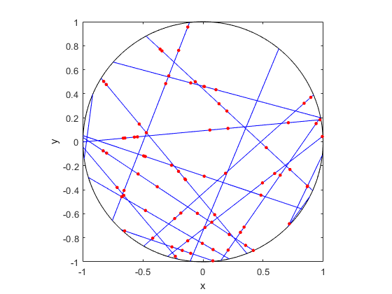
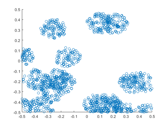
MATLAB

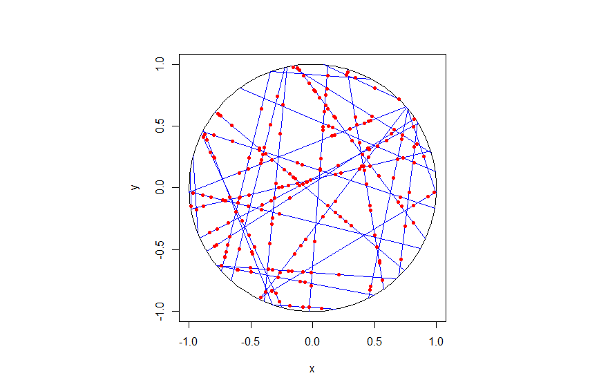
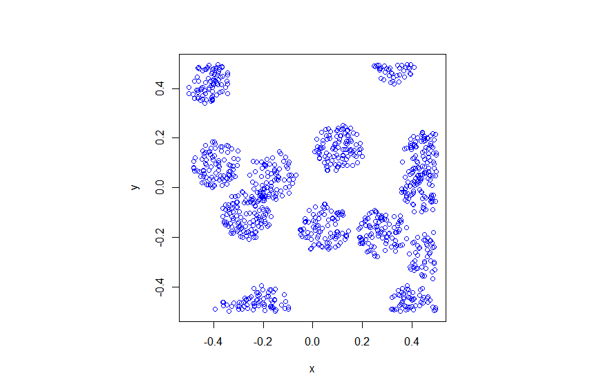
R

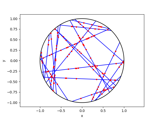
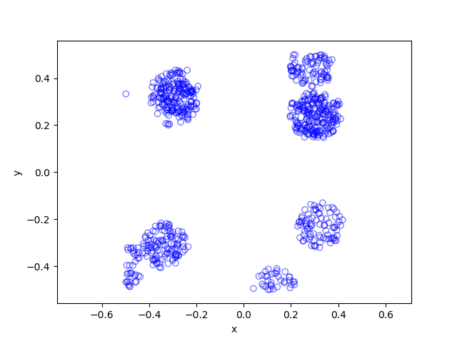
Python

Code

As always, the code from all my posts is online. For this post, I have written the code in MATLAB, R and Python.

Further reading

For the first step, the reading material is basically the same as that for the Poisson line process, which overlaps with that of the Bertrand paradox. For the one-dimensional Poisson point process, we can use the reading material on the homogeneous Poisson point process on a rectangle.

For general Cox point processes, I recommend starting with the following: Chapter 6 in the monograph Poisson Processes by Kingman; Chapter 5 in Statistical Inference and Simulation for Spatial Point Processes by Møller and Waagepetersen; and Section 5.2 in Stochastic Geometry and its Applications by Chiu, Stoyan, Kendall and Mecke. For a much more mathematical treatment, see Chapter 13 in Lectures on the Poisson Process by Last and Penrose, which is freely available online here.

For this particularly Cox point process, see the two aforementioned preprints, located here and here.

Testing the Julia language with point process simulations

I started writing these posts (or blog entries) about a year ago. In my first post I remarked how I wanted to learn to write stochastic simulations in a new language. Well, I found one. It’s called Julia. Here’s my code. And here are my thoughts.

Overview

For scientific programming, the Julia language has arisen as a new contender. Originally started in 2012, its founders and developers have (very) high aspirations, wanting the language to be powerful and accessible, while still having run speeds comparable to C. There’s been excitement about it, and even a Nobel Laureate in economics, Thomas Sargent, has endorsed it. He co-founded the QuantEcon project, whose website has this handy guide or cheat sheet for commands between MATLAB, Python and Julia.

That guide suggests that Julia’s main syntax inspiration comes from MATLAB. But perhaps its closest (and greatest) competitor in scientific programming languages is Python, which has become a standard language used in scientific programming, particularly in machine learning. Another competitor is the statistics language R, which is popular for data science. But R is not renown for its speed.

As an aside, machine learning is closely related to what many call data science. I consider the two disciplines as largely overlapping with statistics, where their respective emphases are on theory and practice. In these fields, often the languages Python and R are used. There are various websites discussing which language is better, such as this one, which in turn is based on this one. In general, it appears that computer scientists and statisticians respectively prefer using Python and R.

Returning to the Julia language, given its young age, the language is still very much evolving, but I managed to find suitable Julia functions for stochastic simulations. I thought I would try it out by simulating some point processes, which I have done several times before. I successfully ran all my code with Julia Version 1.0.3.

In short, I managed to replicate in (or even translate to) Julia the code that I presented in the following posts:

Simulating a homogeneous Poisson point process on a rectangle

Simulating a Poisson point process on a disk

Simulating a Poisson point process on a triangle

Simulating an inhomogeneous Poisson point process

Simulating a Matérn cluster point process

Simulating a Thomas cluster point process

The Julia code, like all the code I present here, can be found on my Github repository, which for this post is located here.

Basics

Language type and syntax

The Wikipedia article on Julia says:

Julia is a high-level general-purpose dynamic programming language designed for high-performance numerical analysis and computational science.

Scientific programming languages like the popular three MATLAB, R and Python, are interpreted languages. But the people behind Julia say:

it is a flexible dynamic language, appropriate for scientific and numerical computing, with performance comparable to traditional statically-typed languages.

Because Julia’s compiler is different from the interpreters used for languages like Python or R, you may find that Julia’s performance is unintuitive at first.

I already remarked that Julia’s syntax is clearly inspired by MATLAB, as one can see in this guide for MATLAB, Python and Julia. But there are key differences. For example, to access an array entry in Julia, you use square brackets (like in most programming languages), whereas parentheses are used in MATLAB or, that old mathematical programming classic, Fortran, which is not a coincidence.

Packages

Julia requires you to install certain packages or libraries, like most languages. For random simulations and plots, you have to install the respective Julia packages Distributions and Plots, which is done by running the code.

Pkg.add("Distributions");
Pkg.add("Plots");

After doing that, it’s best to restart Julia. These packages are loaded with the using command:

Using Distributions;
Using Plots;

Also, the first time it takes a while to run any code using those newly installed packages.

I should stress that there are different plotting libraries. But Plots, which contains many plotting libraries, is the only one I could get working. Another is PlotPy, which uses the Python library. As a beginner, it seems to me that the Julia community has not focused too much on developing new plotting functions, and has instead leveraged pre-existing libraries.

For standard scientific and statistical programming, you will usually also need the packages LinearAlgebra and Statistics.

Data types

Unlike MATLAB or R, Julia is a language that has different data types for numbers, such as integers and floating-point numbers (or floats). This puts Julia in agreement with the clear majority of languages, making it nothing new for most programmers. This is not a criticism of the language, but this can be troublesome if you’ve grown lazy after years of using MATLAB and R.

Simulating random variables

In MATLAB, R and Python, we just need to call a function for simulating uniform, Poisson, and other random variables. There’s usually a function for each type of random variable (or probability distribution).

Julia does simulation of random objects in a more, let’s say, object-oriented way (but I’m told, it’s not an object-oriented language). The probability distributions of random variables are objects, which are created and then sent to a general function for random generation. For example, here’s the code for simulating a Poisson variable with mean \(\mu=10\).

mu=10;
distPoisson=Poisson(mu);
numbPoisson=rand(distPoisson);

Similarly, here’s how to simulate a normal variable with mean \(\mu=10\) and standard deviation \(\sigma=1\).

mu=10;
sigma=1;
distNormal=Normal(mu,sigma);
numbNormal=rand(distNormal);

Of course the last two lines can be collapsed into one.

mu=10;
sigma=1;
numbNormal=rand(Normal(mu,sigma));

But if you just want to create standard uniform variables on the interval (0,1), then the code is like that in MATLAB. For example, this code creates a \(4\times3\) matrix (or array) \(X\) whose entries are simulation outcomes of independent uniform random variables:

X=rand(4,3);

The resulting matrix \(X\) is a Float 64 array.

Arrays

The indexing of arrays in Julia starts at one, just like MATLAB, R, or Fortran. When you apply a function to an array, you generally need to use the dot notation. For example, if I try to run the code:

Y=sqrt(rand(10,1)); #This line will result in an error.

then on my machine (with Julia Version 1.0.3) I get the error:

ERROR: DimensionMismatch(“matrix is not square: dimensions are (10, 1)”)

But this code works:

Y=sqrt.(rand(10,1));

Also, adding scalars to arrays can catch you in Julia, as you also often need to use the dot notation. This code:

Y=sqrt.(rand(10,1));
Z=Y+1; #This line will result in an error.

gives the error:

ERROR: MethodError: no method matching +(::Array{Float64,2}, ::Int64)

This is fixed by adding a dot:

Y=sqrt.(rand(10,1));
Z=Y.+1; #This line will work.

Note the dot has to be on the left hand side. I ended up just using dot notation every time to be safe.

Other traps exist. For example, with indexing, you need to convert floats to integers if you want to use them as indices.

Repeating array elements

There used to be a Julia function called repmat, like the one in MATLAB , but it was merged with a function called repeat. I used such repeating operations to avoid explicit for-loops, which is generally advised in languages like MATLAB and R. For example, I used the repelem function in MATLAB to simulate Matérn and Thomas cluster point processes. To do this in Julia, I had to use this nested construction:

y=vcat(fill.(x, n)...);

This line means that the first value in \(x \) is repeated \(n[1]\) times, where \(n[1]\) is the first entry of \(n\) (as indexing in Julia starts at one), then the second value of \(x\) is repeated \(n[2]\) times, and so on. For example, the vectors \(x=[7,4,9]\) and \(n=[2,1,3]\), the answer is \(y=[7,7,4,9,9,9]\).

To do this in Julia, the construction is not so bad, if you know how, but it’s not entirely obvious. In MATLAB I use this:

y=repelem(x,n);

Similarly in Python:

y=np.repeat(x,n);
Different versions of Julia

I found that certain code would work (or not work) and then later the same code would not work (or would work) on machines with different versions of Julia, demonstrating how the language is still being developed. More specifically, I ran code on Julia Version 1.0.3 (Date 2018-12-18) and Julia Version 0.6.4 (Date: 2018-07-09). (Note how there’s only a few months difference in the dates of the two versions.)

Consider the code with the errors (due to the lack of dot operator) in the previous section. The errors occurred on one machine with Julia Version 1.0.3, but the errors didn’t occur on another machine with the older Julia Version 0.6.4. For a specific example, the code:

Y=sqrt.(rand(10,1));
Z=Y+1; #This line will not result in an error on Version 0.6.4.

gives no error with Julia Version 0.6.4, while I have already discussed how it gives an error with Julia Version 1.0.3.

For another example, I copied from this MATLAB-Python-Julia guide the following command:

A = Diagonal([1,2,3]); #This line will (sometimes?) result in an error.

It runs on machine with Julia Version 0.6.4 with no problems. But running it on the machine with Julia Version 1.0.3 gives the error:

ERROR: UndefVarError: Diagonal not defined

That’s because I have not used the LinearAlgebra package. Fixing this, the following code:

using LinearAlgebra; #Package needed for Diagonal command.
A = Diagonal([1,2,3]); #This line should now work.

gives no error with Julia Version 1.0.3.

If you have the time and energy, you can search the internet and find online forums where the Julia developers have discussed why they have changed something, rendering certain code unworkable with the latest versions of Julia.

Optimization

It seems that performing optimization on functions is done with the Optim package.

Pkg.add("Optim");

But some functions need the Linesearches package, so it’s best to install that as well.

Pkg.add("Linesearches");

Despite those two optimization packages, I ended up using yet another package called BlackBoxOptim.

Pkg.add("BlackBoxOptim");

In this package, I used a function called bboptimize. This is the first optimziation function that I managed to get working. I do not know how it compares to the functions in the Optim and Linesearches packages.

In a previous post, I used optimization functions to simulate a inhomogeneous or nonhomogeneous Poisson point process on a rectangle. I’ve also written Julia code for this simulation, which is found below. I used bboptimize, but I had some problems when I initially set the search regions to integers, which the package did not like, as the values need to be floats. That’s why I multiple the rectangle dimensions by \(1.0\) in the following code:

boundSearch=[(1.0xMin,1.0xMax), (1.0yMin, 1.0yMax)]; #bounds for search box
#WARNING: Values of boundSearch cannot be integers!
resultsOpt=bboptimize(fun_Neg;SearchRange = boundSearch);
lambdaNegMin=best_fitness(resultsOpt); #retrieve minimum value found by bboptimize

Conclusion

In this brief experiment, I found the language Julia good for doing stochastic simulations, but too tricky for doing simple things like plotting. Also, depending on the version of Julia, sometimes my code would work and sometimes it wouldn’t. No doubt things will get better with time.

Further reading

As I said, Julia is still very much an ongoing project. Here’s a couple of links that helped me learn the basics.

https://en.wikibooks.org/wiki/Introducing_Julia/Arrays_and_tuples

https://voxeu.org/content/which-numerical-computing-language-best-julia-matlab-python-or-r

Julia, Matlab, and C

https://modelingguru.nasa.gov/docs/DOC-2676

Code

I’ve only posted here code for some of simulations, but the rest of the code is available on my GitHub repository located here. You can see how the code is comparable to that of MATLAB.

Poisson point process on a rectangle

I wrote about this point process here. The code is located here.

using Distributions #for random simulations
using Plots #for plotting

#Simulation window parameters
xMin=0;xMax=1;
yMin=0;yMax=1;
xDelta=xMax-xMin;yDelta=yMax-yMin; #rectangle dimensions
areaTotal=xDelta*yDelta;

#Point process parameters
lambda=100; #intensity (ie mean density) of the Poisson process

#Simulate Poisson point process
numbPoints=rand(Poisson(areaTotal*lambda)); #Poisson number of points
xx=xDelta*rand(numbPoints,1).+xMin;#x coordinates of Poisson points
yy=yDelta*(rand(numbPoints,1)).+yMin;#y coordinates of Poisson points

#Plotting
plot1=scatter(xx,yy,xlabel ="x",ylabel ="y", leg=false);
display(plot1);
Inhomogeneous Poisson point process on a rectangle

I wrote about this point process here. The code is located here.

using Distributions #for random simulations
using Plots #for plotting
using BlackBoxOptim #for blackbox optimizing

#Simulation window parameters
xMin=-1;xMax=1;
yMin=-1;yMax=1;
xDelta=xMax-xMin;yDelta=yMax-yMin; #rectangle dimensions
areaTotal=xDelta*yDelta;

s=0.5; #scale parameter

#Point process parameters
function fun_lambda(x,y)
    100*exp.(-(x.^2+y.^2)/s^2); #intensity function
end

###START -- find maximum lambda -- START ###
#For an intensity function lambda, given by function fun_lambda,
#finds the maximum of lambda in a rectangular region given by
#[xMin,xMax,yMin,yMax].
#NOTE: Need xMin, xMax, yMin, yMax to be floats eg xMax=1. See boundSearch

function fun_Neg(x)
     -fun_lambda(x[1],x[2]); #negative of lambda
end
xy0=[(xMin+xMax)/2.0,(yMin+yMax)/2.0];#initial value(ie centre)

#Find largest lambda value
boundSearch=[(1.0xMin,1.0xMax), (1.0yMin, 1.0yMax)];
#WARNING: Values of boundSearch cannot be integers!
resultsOpt=bboptimize(fun_Neg;SearchRange = boundSearch);
lambdaNegMin=best_fitness(resultsOpt); #retrieve minimum value found by bboptimize
lambdaMax=-lambdaNegMin;
###END -- find maximum lambda -- END ###

#define thinning probability function
function fun_p(x,y)
    fun_lambda(x,y)/lambdaMax;
end

#Simulate a Poisson point process
numbPoints=rand(Poisson(areaTotal*lambdaMax)); #Poisson number of points
xx=xDelta*rand(numbPoints,1).+xMin;#x coordinates of Poisson points
yy=yDelta*(rand(numbPoints,1)).+yMin;#y coordinates of Poisson points

#calculate spatially-dependent thinning probabilities
p=fun_p(xx,yy);
#Generate Bernoulli variables (ie coin flips) for thinning
booleRetained=rand(numbPoints,1).<p; #points to be retained
xxRetained=xx[booleRetained]; yyRetained=yy[booleRetained];

#Plotting
plot1=scatter(xxRetained,yyRetained,xlabel ="x",ylabel ="y", leg=false);
display(plot1);
Thomas point process on a rectangle

I wrote about this point process here. The code is located here.

using Distributions #for random simulations
using Plots #for plotting

#Simulation window parameters
xMin=-.5;
xMax=.5;
yMin=-.5;
yMax=.5;

#Parameters for the parent and daughter point processes
lambdaParent=10;#density of parent Poisson point process
lambdaDaughter=10;#mean number of points in each cluster
sigma=0.05; #sigma for normal variables (ie random locations) of daughters

#Extended simulation windows parameters
rExt=7*sigma; #extension parameter
#for rExt, use factor of deviation sigma eg 6 or 7
xMinExt=xMin-rExt;
xMaxExt=xMax+rExt;
yMinExt=yMin-rExt;
yMaxExt=yMax+rExt;
#rectangle dimensions
xDeltaExt=xMaxExt-xMinExt;
yDeltaExt=yMaxExt-yMinExt;
areaTotalExt=xDeltaExt*yDeltaExt; #area of extended rectangle

#Simulate Poisson point process
numbPointsParent=rand(Poisson(areaTotalExt*lambdaParent)); #Poisson number of points

#x and y coordinates of Poisson points for the parent
xxParent=xMinExt.+xDeltaExt*rand(numbPointsParent,1);
yyParent=yMinExt.+yDeltaExt*rand(numbPointsParent,1);

#Simulate Poisson point process for the daughters (ie final poiint process)
numbPointsDaughter=rand(Poisson(lambdaDaughter),numbPointsParent);
numbPoints=sum(numbPointsDaughter); #total number of points

#Generate the (relative) locations in Cartesian coordinates by
#simulating independent normal variables
xx0=rand(Normal(0,sigma),numbPoints);
yy0=rand(Normal(0,sigma),numbPoints);

#replicate parent points (ie centres of disks/clusters)
xx=vcat(fill.(xxParent, numbPointsDaughter)...);
yy=vcat(fill.(yyParent, numbPointsDaughter)...);

#Shift centre of disk to (xx0,yy0)
xx=xx.+xx0;
yy=yy.+yy0;

#thin points if outside the simulation window
booleInside=((xx.>=xMin).&(xx.<=xMax).&(yy.>=yMin).&(yy.<=yMax));
#retain points inside simulation window
xx=xx[booleInside];
yy=yy[booleInside];

#Plotting
plot1=scatter(xx,yy,xlabel ="x",ylabel ="y", leg=false);
display(plot1);

Beyond the Poisson point process

As great as the Poisson point process is — and it is pretty great — it is sadly not always suitable for mathematical models. The tractability of this point process is due to the independence of the locations of its points. Informally, this means that point locations of  a Poisson point process in any region will not affect the probability of finding other points in some other region. But such independence may not be true or even approximately true when trying to develop a mathematical model for certain phenomena.

Clustering and Repulsion

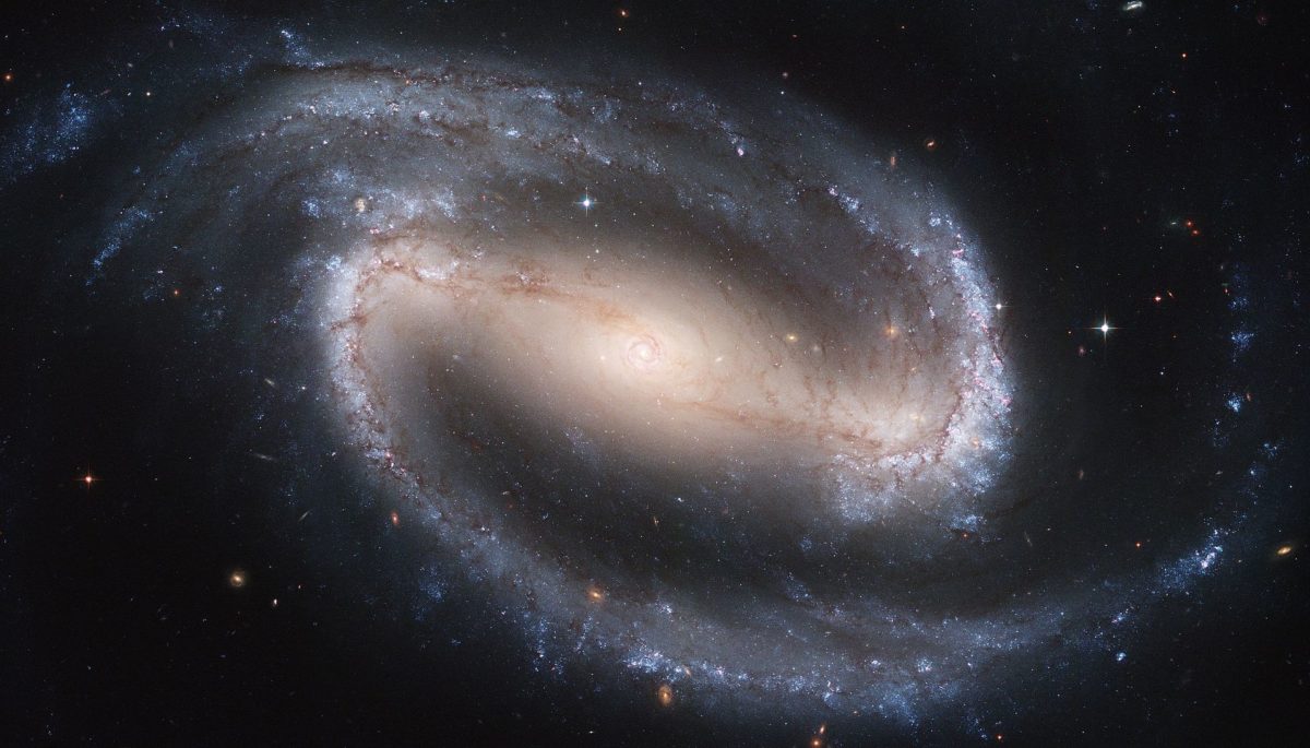
One can quickly think of examples where the Poisson point process is not a suitable model. For example, if a star is part of a galaxy, then it is more likely that another star will be located nearby. Conversely, given the location of a tree in the forest, then usually it is less likely to then find another tree relatively nearby, because trees need a certain amount of land to draw water from the earth.  In the language of point processes, we say that the stars tend to show clustering, while the trees tend to show repulsion.

To better model phenomena like like trees and stars, we can use point processes that also exhibit the properties of clustering and repulsion. In fact, a good part of spatial statistics has been dedicated to developing statistical tools for testing if repulsion or clustering exists in observed point patterns, which is the spatial statistics term used for samples of objects that can be represented as points in space. (A point process is a random object, so a single realization or outcome of a point process is an example of a point pattern.)

The Poisson point process lies halfway between these two categories, meaning that its points show an equal degree of clustering and repulsion. Mathematically, this can be made more formal by, for example, using something called factorial moment measures, which are mathematical objects used to study point processes.

For probability applications, Błaszczyszyn and Yogeshwaran developed a framework using factorial moment measures, which allowed them to classify point process into what they called super-Poisson and sub-Poisson, referring respectively to point processes with points that tend to cluster and repel more.

Point Process Operations

If a Poisson point processes is not suitable for certain models, then we need to develop and use other point processes that exhibit clustering or repulsion. Fortunately, one way to develop such point processes is to apply certain point process operations to Poisson and point processes in general. For developing new point processes, researchers have largely studied three types types of point process operations: thinning, superposition, and clustering. (But there are other operations one can apply to a point process such as randomly moving the points.)

Thinning

To apply the thinning operation means to use some rule for selectively removing points from a point process \(\Phi\) to form a new point process \(\Phi_p\). A rule may be purely random such as the rule known as \(p\)-thinning. For this rule, each point of \(\Phi\) is independently removed (or kept) with some probability \(p\) (or \(1-p\)). This thinning method can be likened to looking at each point, flipping a biased coin with probability \(p\) for heads, and removing the point if a head occurs.

This rule may be generalized by introducing a non-negative function \(p(x)\leq 1\), where \(x\) is a point in the space on which the point process is defined.  This allows us to define a location-dependent \(p(x)\)-thinning, where now the probability of a point being removed is \(p(x)\) and is dependent on where the point \(x\) of \(\Phi\) is located on the underlying space.

The thinning operation is very useful, and I will write more about it in another post, including some examples implemented in code.

Superposition

The superposition of two or more point processes simply means taking the union of two or more point processes. (Point processes can be considered as random sets, which is why point process notation consists of notation from set theory, as well as other mathematical branches.)

More formally, if there is a countable collection of point processes \(\Phi_1,\Phi_2\dots\), then their superposition
\[
\Phi=\bigcup_{i=1}^{\infty}\Phi_i,
\]
also forms a point process. If the point processes are all independent and Poisson, then the superposition will be another Poisson point process, meaning we have not produced a new point process.

Clustering

Related to superposition is a point operation known as clustering, which entails replacing every point \(x\) in a given point process \(\Phi\) with a cluster of points \(N^x\). Each cluster is also a point process, but with a finite number of points. The union of all the clusters forms a cluster point process,  that is
\[
\Phi_c=\bigcup_{x\in \Phi}N^x.
\]

In two previous blogs I have already used this point process operation to construct the Matérn and Thomas (cluster) point processes, which both involve using an underlying Poisson point process. Each point of this point process was assigned a Poisson random number of points, and then the points were uniformly scattered on a disk (for Matérn) or scattered according to a two-dimensional normal distribution (for Thomas). They are members of a family of point processes called Neyman-Scott point processes.

Clustering or repulsion?

I mentioned earlier that in spatial statistics there are statistical tools for testing if clustering or repulsion exists in observed point patterns, usually by comparing it to the Poisson point process, which often serves as a benchmark. For example, in spatial statistics the second factorial moment measure is used for the descriptive statistic called Ripley’s \(K\)-function and its rescaled version, Ripley’s \(L\)-function. Keeping with the alphabetical theme, another example of such a statistic is the \(J\)-function, which was introduced by Van Lieshout and Baddeley.

Further reading

For spatial statistics in general, I always recommend the book Spatial Point Patterns: Methodology and Applications with R written by spatial statistics experts Baddeley, Rubak and Turner, which covers the spatial statistics (and point process simulation) R-package spatstat. This book covers statistically testing point patterns to see if they exhibit more clustering or repulsion, with details for the relevant functions in  spatstat.  For an introduction on factorial moment framework by Błaszczyszyn and Yogeshwaran for clustering and repulsion comparison, see this chapter from a published collection of of lecture notes.

In Chapter 5 of the classic text Stochastic Geometry and its Applications by Chiu, Stoyan, Kendall and Meck, the point process operations thinning are described and used to construct new point processes.  The similar material is covered in the previous edition by Stoyan, Kendall and Mecke.

On a more theoretical level, operations of point processes are covered in the second volume of An Introduction to the Theory of Point Processes by Daley and Vere-Jones. (These convergence results are now a little dated, because there are now various convergence results for point processes based on Stein’s method, which are not included in the book.)

See the previous posts for details and citations on the  Matérn and Thomas (cluster) point processes.

Simulating a Matérn cluster point process

A Matérn cluster point process is a type of cluster point process, meaning that its randomly located points tend to form random clusters. (I skip the details here, but by using techniques from spatial statistics, it is possible to make the definition of clustering more precise.) This point process is an example of a family of cluster point processes known as Neyman-Scott point processes, which have been used in spatial statistics and telecommunications.

I should point out that the Matérn cluster point process should not be confused with the Matérn hard-core point process, which is a completely different type of point process. (For a research article, I have actually written code in MATLAB that simulates this type of point process.) Bertril Matérn proposed at least four types of point processes, and his name also refers to a specific type of covariance function used to define Gaussian processes.

Overview

Simulating a Matérn cluster point process requires first simulating  a homogeneous Poisson point process with an intensity \(\lambda>0\) on some simulation window, such as a rectangle, which is the simulation window I will use here. Then for each point of this underlying point process, simulate a Poisson number of points with mean \(\mu>0\) uniformly on a disk with a constant radius \(r>0\). The underlying  point process is sometimes called the parent (point) process, and its points are centres of the cluster disks.

The subsequent point process on all the disks is called daughter (point) process and it forms the clusters. I have already written about simulating the homogeneous Poisson point processes on a rectangle and a disk, so those posts are good starting points, and I will not focus  too much on details for these steps.

Edge effects

The main challenge behind sampling this point process, which I originally forgot about in an earlier version of this post, is that it’s possible for daughter points to appear in the simulation window that come from parents points outside the simulation window. In other words, parents points outside the simulation window contribute to points inside the window.

To remove these edge effects, the point processes must be simulated on an extended version of the simulation window. Then only the daughter points within the simulation window are kept and the rest are removed.  Consequently, the points are simulated on an extended window, but we only see the points inside the simulation window.

To create the extended simulation window, we can add a strip of width \(r\) all around the simulation window. Why? Well, the distance \(r\) is the maximum distance from the simulation window that a possibly contributing parent point (outside the simulation window) can exist, while still having daughter points inside the simulation window. This means it is impossible for a hypothetical parent point beyond this distance (outside the extended window) to generate a daughter point that can fall inside the simulation window. 

Steps

Number of points

Simulate the underlying or parent Poisson point process on the rectangle with \(N_P\) points. Then for each point, simulate a Poisson number of points, where each disk now has \(D_i\) number of points. Then the total number of points is simply \(N=D_1+\dots +D_{P}=\sum_{i=1}^{N_P}D_i \). The random variables \(P\) and \(D_i\) are Poisson random variables with respective means \(\lambda A\) and \(\mu\), where \(A\) is the area of the rectangular simulation window. To simulate these random variables in MATLAB, use the poissrnd function. To do this in R, use the  standard function rpois. In Python, we can use either functions scipy.stats.poisson or numpy.random.poisson from the SciPy or NumPy libraries.

Locations of points

The points of the parent point process are randomly positioned by using Cartesian coordinates. For a homogeneous Poisson point process, the \(x\) and \(y\) coordinates of each point are independent uniform points, which is also the case for the binomial point process, covered in a previous post. The points of all the daughter point process are randomly positioned by using polar  coordinates. For a homogeneous Poisson point process, the \(\theta\) and \(\rho\) coordinates of each point are independent  variables,  respectively with uniform and triangle distributions, which was covered in a previous post. Then we  convert coordinates back to Cartesian form, which is easily done in MATLAB with the pol2cart function. In languages without such a function: \(x=\rho\cos(\theta)\) and \(y=\rho\sin(\theta)\).

Shifting all the points in each cluster disk

In practice (that is, in the code), all the daughter points are simulated in a disk with its centre at the origin. Then for each cluster disk, all the points have to be shifted to the origin is the center of the cluster, which completes the simulation step.

To use vectorization in the code,  the coordinates of each cluster point are repeated by the number of daughters in the corresponding cluster by using the functions repelem in MATLAB, rep in R, and repeat in Python. 

Code

I’ll now give some code in MATLAB, R and Python, which you can see are all very similar. It’s also located here.

MATLAB

The MATLAB code is located here.

R

The R code is located here.

Of course, as I have mentioned before, simulating a spatial point processes in R is even easier with the powerful spatial statistics library spatstat. The Matérn cluster point process is simulated by using the function rMatClust, but other cluster point processes, including Neyman-Scott types, are possible.

Python

The Pyhon code is located here.

Note: in previous posts I used the SciPy functions for random number generation, but now use the NumPy ones, but there is little difference, as SciPy builds off NumPy.

Julia 

After writing this post, I later wrote the code in Julia. The code is here and my thoughts about Julia are here.

Results

MATLAB

R

Python  

Further reading

Matérn cluster point processes and more generally Neyman-Scott point processes are covered in standard books on the related fields of spatial statistics, point processes and stochastic geometry, such as the following: Spatial Point Patterns: Methodology and Applications with R by  Baddeley, Rubak and Turner, on page 461; Statistical Analysis and Modelling of Spatial Point Patterns Statistics by Illian, Penttinen, Stoyan, amd Stoyan, Section 6.3.2, starting on page 370; Stochastic Geometry and its Applications by Chiu, Stoyan, Kendall and Mecke,  on page 173; and; Statistical Inference and Simulation for Spatial Point Processes by Moller and Waagepetersen, in Section 5.3. I would probably recommend the first two books for beginners.

The Matérn point process has also appeared in models of wireless networks, which we covered in the book Stochastic Geometry Analysis of Cellular Networks by Błaszczyszyn, Haenggi, Keeler, and Mukherjee, Section 8.1.8.

I mentioned above the book Spatial Point Patterns: Methodology and Applications with R , which is written by spatial statistics experts Baddeley, Rubak and Turner. It covers the spatial statistics (and point process simulation) R-package spatstat.