

Mathematical paradoxes are results or observations in mathematics that are (seemingly) conflicting, unintuitive, incomprehensible, or just plain bizarre. They come in different flavours, such as those that play with notions of infinity, which means they often make little or no sense in a physical world. Other paradoxes, particularly those in probability, serve as a lesson that the problem needs to be posed in a precise manner. The Bertrand paradox is one of these.
Joseph Bertrand posed the original problem in his 1889 book Calcul des probabilités, which is available online (in French); page 4, Section 5. It’s a great illustrative problem involving simple probability and geometry, so it often appears in literature on the (closely related) mathematical fields of geometric probability and integral geometry.
Based on constructing a random chord in a circle, Bertrand’s paradox involves a single mathematical problem with three reasonable but different solutions. It’s less a paradox and more a cautionary tale. It’s really asking the question: What exactly do you mean by random?
Consequently, over the years the Bertrand paradox has inspired debate, with papers arguing what the true solution is. I recently discovered it has even inspired some passionate remarks on the internet; read the comments at www.bertrands-paradox.com.
Update: The people from Numberphile and 3Blue1Brown have recently produced a video on YouTube describing and explaining the Bertrand paradox.
But I am less interested in the different interpretations or philosophies of the problem. Rather, I want to simulate the three solutions. This is not very difficult, provided some trigonometry and knowledge from a previous post, where I describe how to simulate a (homogeneous) Poisson point process on the disk.
I won’t try to give a thorough analysis of the solutions, as there are much better websites doing that. For example, this MIT website gives a colourful explanation with pizza and fire-breathing monsters. The Wikipedia article also gives a detailed though less creative explanation for the three solutions.
My final code in MATLAB, R and Python code is located here.
The Problem
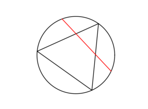
Bertrand considered a circle with an equilateral triangle inscribed it. If a chord in the circle is randomly chosen, what is the probability that the chord is longer than a side of the equilateral triangle?
The Solution(s)
Bertrand argued that there are three natural but different methods to randomly choose a chord, giving three distinct answers. (Of course, there are other methods, but these are arguably not the natural ones that first come to mind.)
Method 1: Random endpoints
On the circumference of the circle two points are randomly (that is, uniformly and independently) chosen, which are then used as the two endpoints of the chord.
The probability of this random chord being longer than a side of the triangle is one third.
Method 2: Random radius
A radius of the circle is randomly chosen (so the angle is chosen uniformly), then a point is randomly (also uniformly) chosen along the radius, and then a chord is constructed at this point so it is perpendicular to the radius.
The probability of this random chord being longer than a side of the triangle is one half.
Method 3: Random midpoint
A point is randomly (so uniformly) chosen in the circle, which is used as the midpoint of the chord, and the chord is randomly (also uniformly) rotated.
The probability of this random chord being longer than a side of the triangle is one quarter.
Simulation
All three answers involve randomly and independently sampling two random variables, and then doing some simple trigonometry. The setting naturally inspires the use of polar coordinates. I assume the circle has a radius \(r\) and a centre at the origin \(o\). I’ll arbitrarily number the end points one and two.
In all three solutions we need to generate uniform random variables on the interval \((0, 2\pi)\) to simulate random angles. I have already done this a couple of times in previous posts such as this one.
Method 1: Random endpoints
This is probably the most straightforward solution to simulate. We just need to simulate two uniform random variables \(\Theta_1\) and \(\Theta_2\) on the interval \((0, 2\pi)\) to describe the angles of the two points.
The end points of the chord (in Cartesian coordinates) are then simply:
Point 1: \(X_1=r \cos \Theta_1\), \(Y_1=r \sin \Theta_1\),
Point 2: \(X_2=r \cos \Theta_2\), \(Y_2=r \sin \Theta_2\).
Method 2: Random radius
This method also involves generating two uniform random variables. One random variable \(\Theta\) is for the angle, while the other \(P\) is the random radius, which means generating the random variable \(P\) on the interval \((0, r)\).
I won’t go into the trigonometry, but the random radius and its perpendicular chord create a right-angle triangle. The distance from the point \((\Theta, P)\) to the circle along the chord is:
$$Q=\sqrt{r^2-P^2}.$$
The endpoints of the chord are then:
Point 1: \(X_1=P \cos \Theta+ Q\sin \Theta\), \(Y_1= P \sin \Theta- Q\cos \Theta\),
Point 2: \(X_2=P \cos \Theta- Q\sin \Theta\), \(Y_2= P \sin \Theta+Q \cos \Theta\).
Take note of the signs in these expressions.
Method 3: Random midpoint
This method requires placing a point uniformly on a disk, which is also done when simulating a homogeneous Poisson point process on a disk, and requires two random variables \(\Theta’\) and \(P’\). Again, the angular random variable \(\Theta’\) is uniform.
The other random variable \(P’\) is not uniform. For \(P’\), we generate a random uniform variable on the unit interval \((0,1)\), and then we take the square root of it. We then multiply it by the radius, generating a random variable between \(0\) and \(r\). (We must take the square root because the area element of a sector is proportional to the radius squared, and not the radius.) The distribution of this random variable is an example of the triangular distribution.
The same trigonometry from Method 2 applies here, which gives the endpoints of the chord as:
Point 1: \(X_1=P’ \cos \Theta’+ Q’\sin \Theta’\), \(Y_1= P’ \sin \Theta’- Q’\cos \Theta’\),
Point 2: \(X_2=P’\cos \Theta’- Q’\sin \Theta’\), \(Y_2= P’\sin \Theta’+Q’ \cos \Theta’\),
where \(Q’:=\sqrt{r^2-{P’}^2}\). Again, take note of the signs in these expressions.
Results
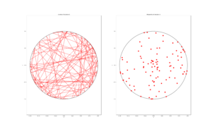
To illustrate how the three solutions are different, I’ve plotted a hundred random line segments and their midpoints side by side. Similar plots are in the Wikipedia article.
Method 1: Random endpoints
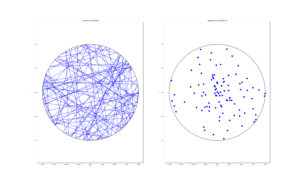
Method 2: Random radius
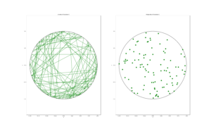
Method 3: Random midpoint
Conclusion
For the chord midpoints, we know and can see that Method 3 gives uniform points, while Method 2 has a concentration of midpoints around the circle centre. Method 1 gives results that seem to somewhere between Method 2 and 3 in terms of clustering around the circle centre.
For the chords, we see that Method 3 results in fewer chords passing through the circle centre. Methods 1 and 2 seem to give a similar number of lines passing through this central region.
It’s perhaps hard to see, but it can be shown that Method 2 gives the most uniform results. By this, I mean that the number of lines and their orientations statistically do not vary in different regions of the circle.
We can now position random lines in uniform manner. All we need now is a Poisson number of lines to generate something known as a Poisson line process, which will be the subject of the next post.
Further reading
I’ve already mentioned that there are some good websites on the topic of the Bertrand paradox. For example:
www.cut-the-knot.org/bertrand.shtml
mathworld.wolfram.com/BertrandsProblem.html
Various authors have mentioned or discussed the Bertrand paradox in books on the related subjects of geometric probability, integral geometry and stochastic geometry. A good and recent introduction is given by Calka in Section 1.3 of the published lectures Stochastic Geometry: Modern Research Frontiers.
Other classic books that cover the topic including, for example, see Problem 1.2 in Geometrical Probability by Kendall and Moran. (Despite Maurice G. Kendall writing a book on geometric probability, he was not related to stochastic geometry pioneer David G Kendall.) It’s also discussed on page 44 in Geometric Probability by Solomon. For a book that involves more advance knowledge of geometry and (abstract) algebra, see Chapter 3 in Integral Geometry and Geometric Probability by Santaló.
The Bertrand paradox is also in The Pleasures of Probability by Isaac. It’s covered in a non-mathematical way in the book Paradoxes from A to Z by Clark. Edwin Jaynes studied the problem and proposed a solution in a somewhat famous 1973 paper, titled The Well-Posed Problem.
The original problem can be read in French in Bertrand’s work, which is available online here or here (starting at the bottom of page 4).
Code
The MATLAB, R and Python code can be found here. In the code, I have labelled the methods A, B and C instead 1, 2 and 3.