Instead of points, we can consider other objects randomly scattered on some underlying mathematical space. If we take a Poisson point process, then we can use (infinitely long) straight lines instead of points, giving a Poisson line process. Researchers have studied and used this random object to model physical phenomena. In this post I’ll cover how to simulate a homogeneous Poisson line process in MATLAB, R and Python. The code can be downloaded from here.
Overview
For simulating a Poisson line process, the key question is how to randomly position the lines. This is related to a classic problem in probability theory called the Bertrand paradox. I discussed this illustration in probability in a previous post, where I also included code for simulating it. I highly recommend reading that post first.
The Bertrand paradox involves three methods for positioning random lines. We use Method 2 to achieve a uniform positioning of lines, meaning the number of lines and orientation of lines is statistically uniform. Then it also makes sense to use this method for simulating a homogeneous (or uniform) Poisson line process.
We can interpret a line process as a point process. For a line process on the plane \(\textbf{R}^2\), it can be described by a point process on \((0,\infty)\times (0,2\pi)\), which is an an infinitely long cylinder. In other words, the Poisson line process can be described as a Poisson point process.
For simulating a Poisson line process, it turns out the disk is the most natural setting. (Again, this goes back to the Bertrand paradox.) More specifically, how the (infinitely long) lines intersect a disk of a fixed radius \(r>0\). The problem of simulating a Poisson line process reduces to randomly placing chords in a disk. For other simulation windows in the plane, we can always bound any non-circular region with a sufficiently large disk.
Steps
Number of lines
Of course, with all things Poisson, the number of lines will be a Poisson random variable, but what will its parameter be? This homogeneous (or uniform) Poisson line process forms a one-dimensional homogeneous (or uniform) Poisson point process around the edge of the disk with a circumference \(2 \pi r \). Then the number of lines is simply a Poisson variable with parameter \(\lambda 2 \pi r \).
Locations of points
To position a single line uniformly in a disk, we need to generate two uniform random variables. One random variable gives the angle describing orientation of the line, so it’s a uniform random variable \(\Theta\) on the interval \((0,2\pi)\).
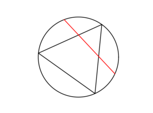
The other random variable gives the distance from the origin to the disk edge, meaning it’s a uniform random variable \(P\) on the interval \((0,r)\), where \(r\) is the radius of the disk. The random radius and its perpendicular chord create a right-angle triangle. The distance from the point \((\Theta, P)\) to the disk edge (that is, the circle) along the chord is:
$$Q=\sqrt{r^2-P^2}.$$
The endpoints of the chord (that is, the points on the disk edge) are then:
Point 1: \(X_1=P \cos \Theta+ Q\sin \Theta\), \(Y_1= P \sin \Theta- Q\cos \Theta\),
Point 2: \(X_2=P \cos \Theta- Q\sin \Theta\), \(Y_2= P \sin \Theta+Q \cos \Theta\).
Code
I have implemented the simulation procedure in MATLAB, R and Python, which, as usual, are all very similar. I haven’t put my code here, because the software behind my website keeps mangling it. As always, I have uploaded my code to a repository; for this post, it’s in this directory.
I have written the code in R, but I wouldn’t use it in general. That’s because if you’re using R, then, as I have said before, I strongly recommend using the powerful spatial statistics library spatstat. For a simulating Poisson line process, there’s the function rpoisline.
The chief author of spatstat, Adrian Baddeley, has written various lectures and books on the related topics of point processes, spatial statistics, and geometric probability. In this post, he answered why the angular coordinates have to be chosen uniformly.
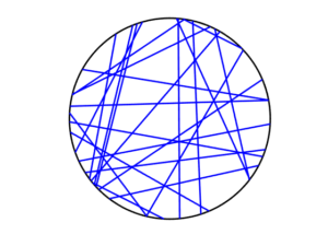
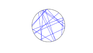
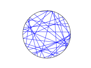
Results
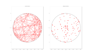
MATLAB
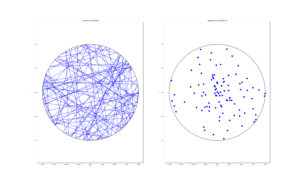
R
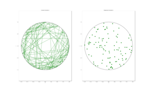
Python
Further reading
To read about the Poisson line process, it’s best to start with the Bertrand problem, which is covered in many works on geometric probability and related fields. A good and recent introduction is given by Calka in (Section 1.3) of the lectures titled Stochastic Geometry: Modern Research Frontiers, which were edited by Coupier and published by Springer. Also see, for example, problem 1.2 in Geometrical Probability by Kendall and Moran or page 44 in Geometric Probability by Solomon.
For the Poisson line process, I highly recommend Section 7.2 in the monograph Poisson Processes by Kingman. Also see Example 8.2 in the standard textbook Stochastic Geometry and its Applications by Chiu, Stoyan, Kendall and Mecke. The Poisson line process book also appears in Exercise 5.2 in the book Stochastic Simulation – Algorithms and Analysis by Asmussen and Glynn.
For online resources, this set of lectures by Christian Lantuéjoul
covers the Poisson line process. Wilfrid Kendall covers the Poisson line process in this talk in relation to so-called Poisson cities.