We can’t all talk all the time, while still being heard. That’s true for people and it’s true for wireless networks.
Networks need to schedule when their network nodes can transmit and receive data. In other words, a collection or subset of network nodes is chosen to transmit, while another subset is chosen to receive. (In telecommunication language, this is part of what is called the medium access control or MAC layer.)
The classic scheduler (spatial)Aloha involves each node flipping a biased coin with probability \(p\) of heads occurring. If heads comes up, a node can transmit. If not, it must stand ready to receive data. Simple.
But can we do better?
Determinantal scheduling
A few years ago, a couple collaborators and I become interested in this problem. To develop an intelligent (or, at least, not stupid) scheduler, we adapted a machine (or statistical) learning framework and published the results in a conference paper:
2020 – Błaszczyszyn, Brochard, and Keeler, Coverage probability in wireless networks with determinantal scheduling.
The hint is in the title. Using a determinantal scheduler, we derived mathematical expressions for the coverage probability. I discussed that paper in an earlier post. I produced the numerical results with code located here and here.
From fermions to generative model
We used a learning framework based on determinantal point process, which were originally used to model subatomic particles called fermions such as electrons. A key property is that determinantal points, like fermions, repel each other, so this is a random model for diversity, anti-clustering or negative correlations.
Defined with a kernel matrix and determinants, these random models have convenient mathematical properties. For example, you can both simulate them (exactly) and train (or fit) them with maximum likelihood methods. Using this fermion model, Kulesa and Taskar proposed and pioneered a machine learning framework.
When properly trained (or fitted), determinantal models can act as generative artificial intelligence (or Gen AI) models. In some sense, these point processes are special types of Gibbsian point processes, which are defined with a general energy function called a Hamiltonian. In the field of AI and computer science more broadly, there are many energy-based models, some of which are used for generative models such as Boltzmann machines.
Recent work
A few days ago I was curious what was happening in this research area, and by chance, I noticed this recently uploaded preprint:
2025 – Tu, Saha, and Dhillon – Determinantal Learning for Subset Selection in Wireless Networks.
I feel more work remains to be done in this area.
Further reading
Wireless networks
Our work was inspired by an earlier paper that we did:
2019 – Błaszczyszyn and Keeler, Determinantal thinning of point processes with network learning applications.
In that paper, which I mentioned in an earlier post, we discussed the potential of using determinantal point processes for scheduling network transmission (or selecting subsets). We pointed out that such a model could be trained on optimized network configurations.
The new work by Tu, Saha, and Dhillon is based on previous work, such as this ambitiously-titled paper:
2019 – Saha and Dhillon – Machine Learning meets Stochastic Geometry: Determinantal Subset Selection for Wireless Networks.
This work by Saha and Dhillon work was independent of our work on scheduling, but came out around the same time.
Machine learning
I should stress that none of the above work was possible without the pioneering efforts by Kulesza and Taskar in a series of papers, much of which appears in their book:
2012 – Kulesza and Taskar – Determinantal point processes for machine learning, Now Publishers.
For those interested in the theory of point processes, Mohamed Karray uploaded some lecture slides, which are based on the book manuscript:
2024 – Baccelli, Błaszczyszyn, and Karray – Random Measures, Point Processes, and Stochastic Geometry.
I have written about this manuscript in a previous post.
Although both the slides and manuscript lean heavily on the side of mathematical rigour, applications are the driving motivation. For example, the third set of slides cover Palm calculus, which hinges upon the important concept of conditioning on a point (of the random point process) existing at a specific location. This idea is frequently used in mathematical models of wireless telecommunication networks based on stochastic geometry. (Unfortunately the Wikipedia article on Palm calculus is sorely lacking and only looks at the temporal, not spatial, setting.)
Karray, a researcher at Orange Labs in Paris, also has slides and (mostly forthcoming) manuscripts on machine learning and statistics, which take a rather rigorous route. It’s a French touch, mathematically, as measure theory appears.
The binomial point process is arguably the simplest point process. It consists of a non-random number of points scattered randomly and independently over some bounded region of space. In this post I will describe the binomial point process, how it leads to the Poisson point process, and its historical role as stars in the sky.
The binomial point process is an important stepping stone in the theory of point process. But I stress that for mathematical models, I would always use a Poisson point process instead of a binomial one. The only exception would be if you were developing a model for a small, non-random number of points.
Uniform binomial point process
We start with the simplest binomial point process, which has uniformly located points. (I described simulating this point process in an early post. The code is here.)
Definition
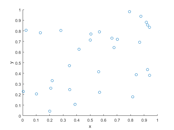
Consider some bounded (or more precisely, compact) region, say, \(W\), of the plane plane \(\mathbb{R}^2\), but the space can be more general. The uniform binomial point process is created by scattering \(n\) points uniformly and independently across the set \(W\).
A single realization of a binomial point process with n=30 points. The points are uniformly and independently scattered across a unit square.
Distribution
Consider a single point uniformly scattered in the region \(W\), giving a binomial point process with \(n=1\). We look at some region \(B\), which is a subset of \(W\), implying \(B\subseteq W\). What is the probability that the single point \(X\) falls in region \(B\)?
First we write \(\nu(W)\) and \(\nu(B)\) to denote the respective areas (or more precisely, Lebesgue measures) of the regions \(W\) and \(B\), hence \(\nu(B)\leq \nu(W)\). Then this probability, say, \(p\), is simply the ratio of the two areas, giving
$$p= P(X\in B)=\frac{\nu(B)}{\nu(W)}.$$
The event of a single point being found in the set \(B\) is a single Bernoulli trial, like flipping a single coin. But if there are \(n\) points, then there are \(n\) Bernoulli trials, which bring us to the binomial distribution.
For a uniform binomial point process \(N_W\), the number of randomly located points being found in a region \(B\) is a binomial random variable, say, \(N_W(B)\), with probability parameter \(p=\nu(B)/ \nu(W)\). The probability mass function of \(N_W(B)\) is
A standard exercise in introductory probability is deriving the Poisson distribution by taking the limit of the binomial distribution. This is done by sending \(n\) (the total number of Bernoulli trials) to infinity while keeping the binomial mean \(\mu:=p n\) fixed, which sends the probability \(p=\mu/n\) to zero.
More precisely, for \(\mu\geq0\), setting \(p_n=\mu/n \) and keeping \(\mu :=p_n n\) fixed, we have the limit result
We can make the same limit argument with the binomial point process.
Homogeneous Poisson point process
We consider the intensity of the uniform binomial point process, which is the average number of points in a unit area. For a binomial point process, this is simply
$$\lambda := \frac{n}{\nu(W)}.$$
For the Poisson limit, we expand the region \(W\) so it covers the whole plane \(\mathbb{R}^2\), while keeping the intensity \(\lambda = n/\nu(W)\) fixed. This means that the area \(\nu(W)\) approaches infinity while the probability \(p=\nu(B)/\nu(W)\) goes to zero. Then in the limit we arrive at the homogeneous Poisson point process \(N\) with intensity \(\lambda\).
The number of points of \(N\) falling in the set \(B\) is a random variable \(N(B)\) with the probability mass function
Typically in point process literature, one first encounters the uniform binomial point process. But we can generalize it so the points are distributed according to some general distribution.
Definition
We write \(\Lambda\) to denote a non-negative Radon measure on \(W\), meaning \(\Lambda(W)< \infty\) and \(\Lambda(B)\geq 0\) for all (measurable) sets \(B\subseteq W\). We can also assume a more general space for the underlying space such as a compact metric space, which is (Borel) measurable. But the intuition still works for compact region of the plane \(\mathbb{R}^2\).
For the \(n\) points, we assume each point is distributed according to the probability measure
$$\bar{\Lambda}= \frac{\Lambda}{\Lambda(W)}.$$
The resulting point process is a general binomial point process. The proofs for this point process remain essentially the same, replacing the Lebesgue measure \(\nu\), such as area or volume, with the non-negative measure \(\Lambda\).
Example
A typical example of the intensity measure \(\Lambda\) has the form
$$\Lambda(B)= \int_B f(x) dx\,,$$
where \(f\) is a non-negative density function on \(W\). Then the probability density of a single point is
$$ p(x) = \frac{1}{c}f(x),$$
where \(c\) is a normalization constant
$$c= \int_W f(x) dx\,.$$
On a set \(W \subseteq \mathbb{R}^2\) using Cartesian coordinates, a specific example of the density \(f\) is
$$ f(x_1,x_2) = \lambda e^{-(x_1^2+x_2^2)}.$$
Distribution
Assuming a general binomial point process \(N_W\) on \(W\), we can use the previous arguments to obtain the binomial distribution
We can easily adapt the Poisson limit arguments for the general binomial Poisson point process, which results in the general Poisson point process \(N\) with intensity measure \(\Lambda\). The number of points of \(N\) falling in the set \(B\) is a random variable \(N(B)\) with the probability mass function
The uniform binomial point process is an example of a spatial point process. With points being scattered uniformly and independently, its sheer simplicity makes it a natural choice for an early spatial model. But which scattered objects?
Perhaps not surprisingly, it is trying to understand star locations where we find the earliest known example of somebody describing something like a random point process. In 1767 in England John Michell wrote:
what it is probable would have been the least apparent distance of any two or more stars, any where in the whole heavens, upon the supposition that they had been scattered by mere chance, as it might happen
As an example, Michelle studied the six brightest stars in the Pleiades star cluster. He concluded the stars were not scattered by mere chance. Of course “scattered by mere chance” is not very precise in today’s probability language, but we can make the reasonable assumption that Michell meant the points were uniformly and independently scattered.
Years later in 1860 Simon Newcomb examined Michell’s problem, motivating him to derive the Poisson distribution as the limit of the binomial distribution. Newcomb also studied star locations. Stephen Stigler considers this as the first example of applying the Poisson distribution to real data, pre-dating the famous work by Ladislaus Bortkiewicz who studied rare events such as deaths from horse kicks. We also owe Bortkiewicz the terms Poisson distribution and stochastic (in the sense of random).
Code
Here, on my repository, are some pieces of code that simulate a uniform binomial point process on a rectangle.
Further reading
For an introduction to spatial statistics, I suggest the lectures notes by Baddeley, which form Chapter 1 of these published lectures, edited by Baddeley, Bárány, Schneider, and Weil. The binomial point process is covered in Section 1.3.
The binomial point process is also covered briefly in the classic text Stochastic Geometry and its Applications by Chiu, Stoyan, Kendall and Mecke; see Section 2.2. Similar material is covered in the book’s previous edition by Stoyan, Kendall and Mecke.
Haenggi also wrote a readable introductory book called Stochastic Geometry for Wireless networks, where he gives the basics of point process theory. The binomial point process is covered in Section 2.4.4.
For some history on point processes and the Poisson distribution, I suggest starting with the respective papers:
Guttorp and Thorarinsdottir, What Happened to Discrete Chaos, the Quenouille Process, and the Sharp Markov Property?;
Stigler, Poisson on the Poisson distribution.
Histories of the Poisson distribution and the Poisson point process are found in the books:
Haight, Handbook of the Poisson Distribution, Chapter 9;
Here’s a lazy summary post where I list all the posts on various Poisson simulations. I’ve also linked to code, which is found on this online repository. The code is typically written in MATLAB and Python.
In the previous post I outlined how to simulate or sample a homogeneous Poisson point process on the surface of a sphere. Now I will consider a homogeneous Poisson point process on the \((n-1)-\) sphere, which is the surface of the Euclidean ball in \(n\) dimensions.
This is a short post because it immediately builds off the previous post. For positioning the points uniformly, I will use Method 2 from that post, which uses normal random variables, as it immediately gives a fast method in \(n\) dimensions.
I wrote this post and the code more for curiosity than any immediate application. But simulating a Poisson point process in this setting requires placing points uniformly on a sphere. And there are applications in that, such as Monte Carlo integration methods, as mentioned in this post, which nicely details different sampling methods.
Steps
As is the case for other shapes, simulating a Poisson point process requires two steps.
Number of points
The number of points of a Poisson point process on the surface of a sphere of radius \(r>0\) is a Poisson random variable. The mean of this random variable is \(\lambda S_{n-1}\), where \(S_{n-1}\) is the surface area of the sphere. For a ball embedded in \(n\) dimension, the area of the corresponding sphere is given by
where \(\Gamma\) is the gamma function, which is a natural generalization of the factorial. In MATLAB, we can simply use the function gamma. In Python, we need to use the SciPy function scipy.special. gamma.
Locations of points
For each point on the sphere, we generate \(n\) standard normal or Gaussian random variables, say, \(W_1, \dots, W_n\), which are independent of each other. These random variables are the Cartesian components of the random point. We rescale the components by the Euclidean norm, then multiply by the radius \(r\).
For \(i=1,\dots, n\), we obtain
$$X_i=\frac{rW_i}{(W_1^2+\cdots+W_n^2)^{1/2}}.$$
These are the Cartesian coordinates of a point uniformly scattered on a sphere with radius \(r\) and a centre at the origin.
How does it work?
In the post on the circle setting, I gave a more detailed outline of the proof, where I said the method is like the Box-Muller transform in reverse. The joint density of the normal random variables is from a multivariate normal distribution with zero correlation. This joint density a function of the Cartesian equation for a sphere. This means the density is constant on the sphere, implying that the angle of the point \((W_1,\dots, W_n)\) will be uniformly distributed.
The vector formed from the normal variables \((W_1,\dots,W_n)\) is a random variable with a chi distribution. But the final vector, which stretches from the origin to the point \((X_1,\dots,X_n)\), has length one, because we rescaled it with the Euclidean norm.
Code
The code for all my posts is located online here. For this post, the code in MATLAB and Python is here.
Further reading
I recommend this blog post, which discusses different methods for randomly placing points on spheres and inside spheres (or, rather, balls) in a uniform manner. (Embedded in two dimensions, a sphere is a circle and a ball is a disk.)
Our Method 2 for positioning points uniformly, which uses normal variables, comes from the paper:
1959, Muller, A note on a method for generating points uniformly on n-dimensional spheres.
Two recent works on this approach are the papers:
2010, Harman and Lacko, On decompositional algorithms for uniform sampling from -spheres and -balls;
2017, Voelker, Gosman, Stewart, Efficiently sampling vectors and coordinates.
In this post I’ll describe how to simulate or sample a homogeneous Poisson point process on the surface of a sphere. I have already simulated this point process on a rectangle, triangledisk, and circle.
Of course, by sphere, I mean the everyday object that is the surface of a three-dimensional ball, where this two-dimensional object is often denoted by \(S^2\). Mathematically, this is a generalization from a Poisson point process on a circle, which is slightly simpler than randomly positioning points on a disk. I recommend reading those two posts first, as a lot of the material presented here builds off them.
I have not needed such a simulation in my own work, but I imagine there are many reasons why you would want to simulate a Poisson point process on a sphere. As some motivation, we can imagine these points on a sphere representing, say, meteorites or lightning hitting the Earth.
The generating the number of points is not difficult. The trick is positioning the points on the sphere in a uniform way. As is often the case, there are various ways to do this, and I recommend this post, which lists the main ones. I will use two methods that I consider the most natural and intuitive ones, namely using spherical coordinates and normal random variables, which is what I did in the post on the circle.
Incidentally, a simple modification allows you to scatter the points uniformly inside the sphere, but you would typically say ball in mathematics, giving a Poisson point process inside a ball; see below for details.
Steps
As always, simulating a Poisson point process requires two steps.
Number of points
The number of points of a Poisson point process on the surface of a sphere of radius \(r>0\) is a Poisson random variable with mean \(\lambda S_2\), where \(S_2=4\pi r^2\) is the surface area of the sphere. (In this post I give some details for simulating or sampling Poisson random variables or, more accurately, variates.)
Locations of points
For any homogeneous Poisson point process, we need to position the points uniformly on the underlying space, which is in this case is the sphere. I now outline two different methods for doing this.
Method 1: Spherical coordinates
The first method is based on spherical coordinates \((\rho, \theta,\phi)\), where the radial coordinate \(\rho\geq 0\), and the angular coordinates \(0 \leq \theta\leq 2\pi\) and \(0\leq \phi \leq \pi\). The change of coordinates gives \(x=\rho\sin(\theta)\cos(\phi)\), \(y=\rho\sin(\theta)\sin(\phi)\), and \(z=\rho\cos(\phi)\).
Now we use Proposition 1.1 in this paper by Pitman and Ross. For each point, we generate two uniform variables \(V\) and \(\Theta\) on the respective intervals \((-1,1)\) and \((0,2\pi)\). Then we place the point with the Cartesian coordinates
$$X = r \sqrt{1-V^2} \cos\Theta, $$
$$Y = r \sqrt{1-V^2}\sin\Theta, $$
$$ Z=r V. $$
This method places a uniform point on a sphere with a radius \(r\).
How does it work?
I’ll skip the precise details, but give some interpretation of this method. The random variable \(\Phi := \arccos V\) is the \(\phi\)-coordinate of the uniform point, which implies \(\sin \Phi=\sqrt{1-V^2}\), due to basic trigonometric identities. The area element in polar coordinates is \(dA = \rho^2 \sin\phi d\phi d\theta \), which is constant with respect to \(\theta\). After integrating with respect to \(\phi\), we see that the random variable \(V=\cos\Phi\) needs to be uniform (instead of \(\Phi\)) to ensure the point is uniformly located on the surface.
Method 2: Normal random variables
For each point, we generate three standard normal or Gaussian random variables, say, \(W_x\), \(W_y\), and \(W_z\), which are independent of each other. (The term standard here means the normal random variables have mean \(\mu =0\) and standard deviation \(\sigma=1\).) The three random variables are the Cartesian components of the random point. We rescale the components by the Euclidean norm, then multiply by the radius \(r\), giving
$$X=\frac{rW_x}{(W_x^2+W_y^2+W_z^2)^{1/2}},$$
$$Y=\frac{rW_y}{(W_x^2+W_y^2+W_z^2)^{1/2}},$$
$$Z=\frac{rW_z}{(W_x^2+W_y^2+W_z^2)^{1/2}}.$$
These are the Cartesian coordinates of a point uniformly scattered on a sphere with radius \(r\) and a centre at the origin.
How does it work?
The procedure is somewhat like the Box-Muller transform in reverse. In the post on the circle setting, I gave an outline of the proof, which I recommend reading. The joint density of the normal random variables is from a multivariate normal distribution with zero correlation. This joint density is constant on the sphere, implying that the angle of the point \((W_x, W_y, W_z)\) will be uniformly distributed.
The vector formed from the normal variables \((W_x, W_y,W_z)\) is a random variable with a chi distribution. We can see that the vector from the origin to the point \((X,Y,Z)\) has length one, because we rescaled it with the Euclidean norm.
Plotting
Depending on your plotting software, the points may more resemble points on an ellipsoid than a sphere due to the different scaling of the x, y and z axes. To fix this in MATLAB, run the command: axis square. In Python, it’s not straightforward to do this, as it seems to lack an automatic function, so I have skipped it.
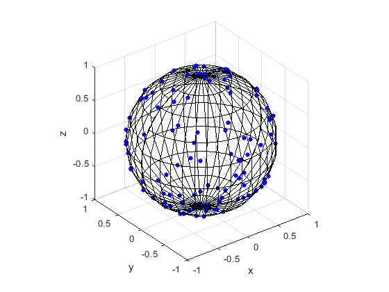
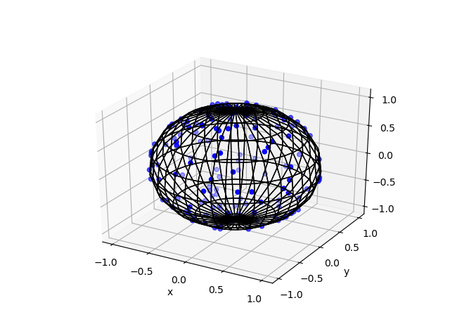
Results
Here are some results produced by code written in MATLAB and Python. The blue points are the Poisson points on the sphere. I have used a surface plot (with clear faces) to illustrate the underling sphere in black.
MATLAB
Python
Note: The aspect ratio in 3-D Python plots tends to squash the sphere slightly, but it is a sphere.
Code
The code for all my posts is located online here. For this post, the code in MATLAB and Python is here. In Python I used the library mpl_toolkits for doing 3-D plots.
Poisson point process inside the sphere
Perhaps you want to simulate a Poisson point process inside the ball. There are different ways we can do this, but I will describe just one way, which builds off Method 1 for positioning the points uniformly. (In a later post, I will modify Method 2, giving a way to uniformly position points inside the ball.)
For this simulation method, you need to make two simple modifications to the simulation procedure.
Number of points
The number of points of a Poisson point process inside a sphere of radius \(r>0\) is a Poisson random variable with mean \(\lambda V_3\), where \(V_3=4\pi r^3\) is the volume of the sphere.
Locations of points
We will modify Method 1 as outlined above. To sample the points uniformly in the sphere, you need to generate uniform variables on the unit interval \((0,1)\), take their cubic roots, and then, multiply them by the radius \(r\). (This is akin to the step of taking the square root in the disk setting.) The random variables for the angular coordinates are generated as before.
Further reading
I recommend this blog post, which discusses different methods for randomly placing points on spheres and inside spheres (or, rather, balls) in a uniform manner. (Embedded in two dimensions, a sphere is a circle and a ball is a disk.)
Our Method 2 for positioning points uniformly, which uses normal variables, comes from the paper:
1959, Muller, A note on a method for generating points uniformly on n-dimensional spheres.
This sampling method relies upon old observations that normal variables are connected to spheres and circles. I also found this post on a similar topic. Perhaps not surprisingly, the above paper is written by the same Muller behind the Box-Muller method for sampling normal random variables.
Update: The connection between the normal distribution and rotational symmetry has been the subject of some recent 3Blue1Brown videos on YouTube.
Here is some sample Python code for creating a 3-D scatter plot.
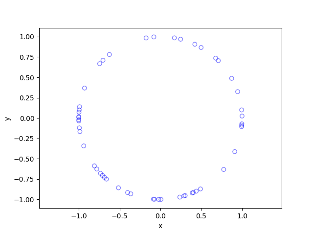
In this post, I’ll take a break from the more theoretical posts. Instead I’ll describe how to simulate or sample a homogeneous Poisson point process on a circle. I have already simulated this point process on a rectangle, triangle and disk. In some sense, I should have done this simulation method before the disk one, as it’s easier to simulate. I recommend reading that post first, as the material presented here builds off it.
Sampling a homogeneous Poisson point process on a circle is rather straightforward. It just requires using a fixed radius and uniformly choose angles from interval \((0, 2\pi)\). But the circle setting gives an opportunity to employ a different method for positioning points uniformly on circles and, more generally, spheres. This approach uses Gaussian random variables, and it becomes much more efficient when the points are placed on high dimensional spheres.
Steps
Simulating a Poisson point process requires two steps: simulating the random number of points and then randomly positioning each point.
Number of points
The number of points of a Poisson point process on circle of radius \(r>0\) is a Poisson random variable with mean \(\lambda C\), where \(C=2\pi r\) is the circumference of the circle. You just need to be able to need to produce (pseudo-)random numbers according to a Poisson distribution.
To generate Poisson variables in MATLAB, use the poissrnd function with the argument \(\lambda C\). In Python, use either the scipy.stats.poisson or numpy.random.poisson function from the SciPy or NumPy libraries. (If you’re curious how Poisson simulation works, I suggest seeing this post for details on sampling Poisson random variables or, more accurately, variates.)
Locations of points
For a homogeneous Poisson point process, we need to uniformly position points on the underlying space, which is this case is a circle. We will look at two different ways to position points uniformly on a circle. The first is arguably the most natural approach.
Method 1: Polar coordinates
We use polar coordinates due to the nature of the problem. To position all the points uniformly on a circle, we simple generate uniform numbers on the unit interval \((0,1)\). We then multiply these random numbers by \(2\pi\).
We have generated polar coordinates for points uniformly located on the circle. To plot the points, we have to convert the coordinates back to Cartesian form by using the change of coordinates: \(x=\rho\cos(\theta)\) and \(y=\rho\sin(\theta)\).
Method 2: Normal random variables
For each point, we generate two standard normal or Gaussian random variables, say, \(W_x\) and \(W_y\), which are independent of each other. (The term standard here means the normal random variables have mean \(\mu =0\) and standard deviation \(\sigma=1\).) These two random variables are the Cartesian components of a random point. We then rescale the two values by the Euclidean norm, giving
$$X=\frac{W_x}{(W_x^2+W_y^2)^{1/2}},$$
$$Y=\frac{W_y}{(W_x^2+W_y^2)^{1/2}}.$$
These are the Cartesian coordinates of points uniformly scattered around a unit circle with centre at the origin. We multiply the two random values \(X\) and \(Y\) by the \(r>0\) for a circle with radius \(r\).
How does it work?
The procedure is somewhat like the Box-Muller transform in reverse. I’ll give an outline of the proof. The joint density of the random variables \(W_x\) and \(W_y\) is that of the bivariate normal distribution with zero correlation, meaning it has the joint density
$$ f(x,y)=\frac{1}{2\pi}e^{[-(x^2+y^2)/2]}.$$
We see that the function \(f\) is a constant when we trace around any line for which \((x^2+y^2)\) is a constant, which is simply the Cartesian equation for a circle (where the radius is the square root of the aforementioned constant). This means that the angle of the point \((W_x, W_y)\) will be uniformly distributed.
Now we just need to look at the distance of the random point. The vector formed from the pair of normal variables \((W_x, W_y)\) is a Rayleigh random variable. We can see that the vector from the origin to the point \((X,Y)\) has length one, because we rescaled it with the Euclidean norm.
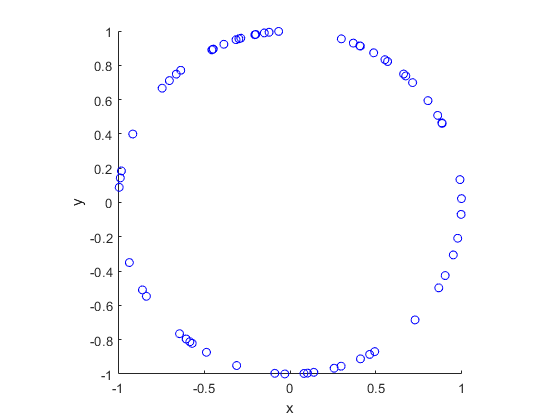
Results
I have presented some results produced by code written in MATLAB and Python. The blue points are the Poisson points on the sphere. I have used a surface plot (with clear faces) in black to illustrate the underling sphere.
MATLAB
Python
Code
The code for all my posts is located online here. For this post, the code in MATLAB and Python is here.
Further reading
I recommend this blog post, which discusses different methods for randomly placing points on spheres and inside spheres (or, rather, balls) in a uniform manner. (Embedded in two dimensions, a sphere is a circle and a ball is a disk.) A key paper on using normal variables is the following:
1959, Muller, A note on a method for generating points uniformly on n-dimensional spheres.
As I mentioned in the post on the disk, the third edition of the classic book Stochastic Geometry and its Applications by Chiu, Stoyan, Kendall and Mecke details on page 54 how to uniformly place points on a disk. It just requires a small modification for the circle.
In previous posts I have often stressed the importance of the Poisson point process as a mathematical model. But it can be unsuitable for certain mathematical models. We can generalize it by first considering a non-negative random measure, called a driving or directing measure. Then a Poisson point process, which is independent of the random driving measure, is generated by using the random measure as its intensity or mean measure. This doubly stochastic construction gives what is called a Cox point process.
In practice we don’t typically observe the driving measure. This means that it’s impossible to distinguish a Cox point process from a Poisson point process if there’s only one realization available. By conditioning on the random driving measure, we can use the properties of the Poisson point process to derive those of the resulting Cox point process.
By the way, Cox point processes are also known as doubly stochastic Poisson point processes. Guttorp and Thorarinsdottir argue that we should call them the Quenouille point processes, as Maurice Quenouille introduced an example of it before Sir David Cox. But I opt for the more common name.
In this post I’ll cover a couple examples of Cox point processes. But first I will need to give a more precise mathematical definition.
Definition
We consider a point process defined on some underlying mathematical space \(\mathbb{S}\), which is sometimes called the carrier space or state space. The underlying space is often the real line \(\mathbb{R}\), the plane \(\mathbb{R}^2\), or some other familiar mathematical space like a square lattice.
For the first definition, we use the concept of a random measure.
Let \(M\) be a non-negative random measure on \(\mathbb{S} \). Then a point process \(\Phi\) defined on some underlying space \(\mathbb{S}\) is a Cox point process driven by the intensity measure \(M\) if the conditional distribution of \(\Phi\) is a Poisson point process with intensity function \(M\).
We can give a slightly less general definition of a Cox point process by using a random intensity function.
Let \(Z=\{Z(x):x\in\mathbb{S} \}\) be a non-negative random field such that with probability one, \(x\rightarrow Z(x)\) is a locally integrable function. Then a point process \(\Phi\) defined on some underlying space \(\mathbb{S}\) is a Cox point process driven by \(Z\) if the conditional distribution of \(\Phi\) is a Poisson point process with intensity function \(Z\).
The random driving measure \(M\) is then simply the integral
$$
M(B)=\int_B Z(x)\, dx , \quad B\subseteq S.
$$
Over-dispersion
The random driving measures take different forms, giving different Cox point processes. But there is a general observation that can be made for all Cox point processes. For any region \(B \subseteq S\), it can be shown that the number of points \(\Phi (B)\) adheres to the inequality
$$
\mathbb{Var} [\Phi (B)] \geq \mathbb{E} [\Phi (B)],
$$
where \(\mathbb{Var} [\Phi (B)] \) is the variance of the random variable \(\Phi (B)\). As a comparison, for a Poisson point process \(\Phi’\), the variance of \(\Phi’ (B)\) is simply \(\mathbb{Var} [\Phi’ (B)] =\mathbb{E} [\Phi’ (B)]\). Due to its greater variance, the Cox point process is said to be over-dispersed compared to the Poisson point process.
Special cases
There is an virtually unlimited number of ways to define a random driving measure, where each one yields a different a Cox point process. But in general we are restricted by examining only tractable and interesting Cox point processes. I will give some common examples, but I stress that the Cox point process family is very large.
Mixed Poisson point process
For the random driving measure \(M\), an obvious example is the product form \(M= Y \mu \), where \(Y\) is some independent non-negative random variable and \(\mu\) is the Lebesgue measure on \(\mathbb{S}\). This driving measure gives the mixed Poisson point process. The random variable \(Y\) is the only source of randomness.
Log-Gaussian Cox point process
Instead of a random variable, we can use a non-negative random field to define a random driving measure. We then have the product \(M= Y \mu \), where \(Y\) is now some independent non-negative random field. (A random field is a collection of random variables indexed by some set, which in this case is the underlying space \(\mathbb{S}\).)
Arguably the most tractable and used random field is the Gaussian random field. This random field, like Gaussian or normal random variables, takes both negative and positive values. But if we define the random field such that its logarithm is a Gaussian field \(Z\), then we obtain the non-negative random driving measure \(M=\mu e^Z \), giving the log-Gaussian Cox point process.
This point process has found applications in spatial statistics.
Cox-Poisson line-point process
To construct this Cox point process, we first consider a Poisson line process, which I discussed previously. Given a Poisson line process, we then place an independent one-dimensional Poisson point process on each line. We then obtain an example of a Cox point process, which we could call a Cox line-point process or a Cox-Poisson line-point process. (But I am not sure of the best name.)
Researchers have recently used this point process to study wireless communication networks in cities, where the streets correspond to Poisson lines. For example, see these two preprints:
We construct the next Cox point process by first considering a Poisson point process on the space \(\mathbb{S}\) to create a shot noise term. (Shot noise is just the sum of some function over all the points of a point process.) We then use it as the driving measure of the Cox point process.
More specifically, we first introduce a kernel function \(k(\cdot,\cdot)\) on \(\mathbb{S}\), where \(k(x,\cdot)\) is a probability density function for all points \(x\in \mathbb{S}\). We then consider a Poisson point process \(\Phi’\) on \(\mathbb{S}\times (0,\infty)\). We assume the Poisson point process \(\Phi’\) has a locally integrable intensity function \(\mu \).
(We can interpret the point process \(\Phi’\) as a spatially-dependent marked Poisson point process, where the unmarked Poisson point process is defined on \(\mathbb{S}\). We then assume each point \(X\) of this unmarked point process has a mark \(T \in (0,\infty)\) with probability density \(\mu(X,t)\).)
The resulting shot noise
$$
Z(x)= \sum_{(Y,T)\in \Phi’} T \, k(Y,x)\,,
$$
gives the random field. We then use it as the random intensity function to drive the shot-noise Cox point process.
In previous posts, I have detailed how to simulate non-Poisson point processes such as the Matérn and Thomas cluster point processes. These are examples of a Neyman-Scott point process, which is a special case of a shot noise Cox point process. All these point processes find applications in spatial statistics.
Simulation
Unfortunately, there is no universal way to simulate all Cox point processes. (And even if there were one, it would not be the most optimal way for every Cox point process.) The simulation method depends on how the Cox point process is constructed, which usually means how its directing or driving measure is defined.
In previous posts I have presented ways (with code) to simulate these Cox point processes:
In addition to the Matérn and Thomas point processes, there are ways to simulate more general shot noise Cox point processes. I will cover that in another post.
When working with random variables, a couple useful tools are the characteristic function and the moment-generating function, which for a random variable \(Y\) are defined respectively as
$$
\phi_Y(t)= \mathbb{E}\left [ e^{itY} \right ]\,
$$
and
$$
M_Y(t)= \mathbb{E}\left [ e^{tY} \right ]\,,
$$
where the imaginary number \(i=\sqrt{-1}\) and the real variable \(t\in \mathbb{R}\). For continuous random variables, these two respective functions are essentially the Fourier and Laplace transforms of the probability densities. (The moment-generating function \(M(t)\) may not exist due to the integral not converging to a finite value, whereas the characteristic function \(\phi_Y(t)\) always exists.)
If \(Y\) is a discrete random variable, a useful object is the probability-generating function, which is defined as
$$
G_Y(z)= \mathbb{E}\left [z^Y \right ]\,.
$$
This function is the Z-transform of the probability mass function of the random variable \(Y\).
By using these tools, results such as sums of random variables and convergence theorems can be proven. There exist equivalent tools which prove useful for studying point processes (and, more generally random measures).
Laplace functional
For a point process \(\Phi \) defined on some underlying space \(\mathbb{S}\), such as \(\mathbb{R}^d\), the Laplace functional is defined as
$$
L_{\Phi}(f)=\mathbb{E}[e^{-\int_{ \mathbb{S}} f(x){\Phi}(dx)}]\,,
$$
where \(f\) is any (Borel) measurable non-negative function on the space \(\mathbb{S}\).
A simple point process is one for which two or more points coincide in location with probability zero. For a simple point process, we can write the random integral (or sum) using set theory notation, giving
$$
\int_{\mathbb{S}} f(x){\Phi}(dx)=\sum\limits_{x\in \Phi} f(x) \,.
$$
Name
Why’s it called a Laplace functional? From its definition, it’s clear that the first half of the name stems from the Laplace transform. Mapping from the space \(\mathbb{S}\), it’s called a functional because it is a function of a non-negative function \(f\).
Characterization
The Laplace functional characterizes the point process, meaning each point process (or, more generally, random measure) has its own unique Laplace functional. For a given point process, the challenge is to derive the mathematical expression for the Laplace functional by using its definition.
Poisson example
For deriving the Laplace functional, perhaps not surprisingly, one of the easiest one of the easiest point processes is the Poisson point process due to its independence property. For a Poisson process \(\Phi\) with intensity measure \(\Lambda\) defined on the state space \(\mathbb{S}\), the Laplace functional is given by
$$
L_{\Phi}(f)=e^{-\int_{ \mathbb{S}} [1-e^{-f(x)}]\,\Lambda(dx) } \,.
$$
where \(\lambda\) is the intensity function (that is, the average density of points).
Applications
Proof techniques
Given a Laplace functional characterizes a point process, it can be used prove results on the distributions of point processes, where the proofs often simpler. For example, it can used to see what happens when you perform a point process operation on a point process, such as proving that the independent thinning a Poisson point process gives another Poisson point process. Laplace functionals are used to prove results on the superposition and (random or deterministic) mapping of point processes.
Interference in wireless network models
In the previous post, I covered the concept of the signal-to-interference ratio or SIR in wireless networks. (If noise is included, then then signal-to-interference-plus-noise ratio or just SINR.) Under such wireless network models, the interference term is a type of shot noise of the point process used for the transmitter locations.
Researchers commonly assume Rayleigh fading of the signal energy, which corresponds to the power values randomly varying according to an exponential distribution (due to a square root being taken). The tail distribution of an exponential variable \(F\) with mean \(\mu\) is simply \(\mathbb{P}(F>t)= e^{-t/\mu}\). This means that the exponential assumption and some conditioning arguments lead to Laplace transforms of random variables, including the interference, which can be recast as the Laplace functional of the point process used for the transmitter locations.
Related functionals
For random variables, the characteristic, moment-generating, and probability-generating functions are similarly defined and closely related. We now define two other functionals used for studying point processes.
Characteristic functional
For a point process \(\Phi \) defined on \(\mathbb{S}\), the characteristic functional is defined as
$$
L_{\Phi}(f)=\mathbb{E}[e^{i\int_{ \mathbb{S}} g(x){\Phi}(dx)}]\,,
$$
where \(i=\sqrt{-1}\) and \(g\) is any (Borel) measurable function on the space \(\mathbb{S}\).
Probability-generating functional
For a point process \(\Phi \) defined on \(\mathbb{S}\), the probability-generating functional is defined as
$$
G_{\Phi}(v)=\mathbb{E}[ \prod_{x\in \Phi } v(x)]\,,
$$
where \(v\) is any bounded non-negative (Borel) measurable function on the space \(\mathbb{S}\) such that \(0\leq v(x)\leq 1\) for any point \(x\in \mathbb{S}\). (Some authors use an alternative definition with a function \(u(x)=1-v(x)\).)
The usual sources on point processes (and, more generally, random measures) cover Laplace functionals. For example, see section 7.2.1 of the text Stochastic Geometry and its Applications by Chiu, Stoyan, Kendall and Mecke. The Laplace and other functionals are covered in Section 9.4 of the second volume of An Introduction to the Theory of Point Processes by Daley and Vere-Jones.
In a previous post, I wrote about the concept of shot noise of a point process. In the simplest terms, shot noise is just the sum of some function over all the points of a point process. The name stems from the original mathematical models of the noise in old electronic devices, which was compared to shot (used in guns) hitting a surface.
In this post I will present a result known as Campbell’s theorem or Campbell’s formula, which gives the expectation of shot noise as as simple integral expression. This both a general holding for all point processes. It is also useful, as shot noise naturally arises in mathematical models. One application is wireless network models, where the interference term is shot noise.
But to present the main result, I first need to give some basics of point processes, most of which I already covered in this post.
Point process basics
We consider a point processes \(\Phi\) defined on some underlying mathematical space \(\mathbb{S}\), which is often \(\mathbb{R}^n\). Researchers typically interpret a point process as a random counting measure, resulting in the use of integral and measure theory notation. For example, \(\Phi(B)\) denotes the number of points located in some (Borel measurable) set \(B\), which is a subset of \(\mathbb{S}\).
For point processes, researchers often use a dual notation such that \(\Phi\) denotes both a random set or a random measure. Then we can write, for example, \(\Phi=\{X_i\}_i\) to stress that \(\Phi\) is a random sets of points. (Strictly speaking, you can only use the set notation if the point process is simple, meaning that no two points coincide with probability one.)
The first moment measure of a point process, also called the mean measure or intensity measure, is defined as
$$\Lambda(B)= \mathbb{E} [\Phi(B)]. $$
In other words, the first moment measure can be interpreted as the expected number of points of \(\Phi\) falling inside the set \(B \subseteq \mathbb{S}\).
Shot noise definition
We assume a point process \(\Phi=\{X_i\}_i\) is defined on some space \(\mathbb{S}\). We consider a non-negative function \(f\) with the domain \(\mathbb{S}\), so \(f:\mathbb{S} \rightarrow [0,\infty)\). If the point process \(\Phi\) is a simple, we can use set notation and define the shot noise as
$$
S= \sum_{X_i\in \Phi} f(X_i)\,.
$$
More generally, the shot noise is defined as
$$
S= \int_{ \mathbb{S}} f(x) \Phi(dx)\,.
$$
(We recall that an integral is simply a more general type of sum, which is why the integral sign comes from the letter S.)
Campbell’s theorem
We now state Campbell’s theorem.
Campbell’s theorem says that for any point process \(\Phi\) defined on a space \(\mathbb{S}\) the following formula holds
where \(\Lambda= \mathbb{E} [\Phi(B)]\) is the intensity measure of the point process \(\Phi\).
Interpretation
The integral formula is just an application of Fubini’s theorem, as we have simply changed the order of integration. The formula holds for general processes because it is simply a result on first moments, so it is leveraging the linearity of sums and integrals, including the expectation operator. Put more simply, the sum of parts does equal the whole.
Some history
At the beginning of the 20th century, Norman R. Campbell studied shot noise in Britain and wrote two key papers. In one of these papers appears a version of the result we now called Campbell’s theorem or Campbell’s formula. Interestingly, Campbell was a physicist who credited his mathematical result to renown pure mathematician G. H. Hardy. Hardy claimed years later that, given he only researched pure mathematics, none of his work would lead to applications. But Hardy’s claim is simply not true due to this result, as well as his results in number theory, which are famously used in modern day cryptography.
Further reading
For some basics on point processes, I suggest the classic text Stochastic Geometry and its Applications by Chiu, Stoyan, Kendall and Mecke, which covers point processes and the varying notation in Chapters 2 and 4. Haenggi also wrote a very readable introductory book called Stochastic Geometry for Wireless networks, where he gives the basics of point process theory.
These moment formula are also presented with proofs in Applied Probability by Lange; see Section 6.9.