I started writing these posts (or blog entries) about a year ago. In my first post I remarked how I wanted to learn to write stochastic simulations in a new language. Well, I found one. It’s called Julia. Here’s my code. And here are my thoughts.
Overview
For scientific programming, the Julia language has arisen as a new contender. Originally started in 2012, its founders and developers have (very) high aspirations, wanting the language to be powerful and accessible, while still having run speeds comparable to C. There’s been excitement about it, and even a Nobel Laureate in economics, Thomas Sargent, has endorsed it. He co-founded the QuantEcon project, whose website has this handy guide or cheat sheet for commands between MATLAB, Python and Julia.
That guide suggests that Julia’s main syntax inspiration comes from MATLAB. But perhaps its closest (and greatest) competitor in scientific programming languages is Python, which has become a standard language used in scientific programming, particularly in machine learning. Another competitor is the statistics language R, which is popular for data science. But R is not renown for its speed.
As an aside, machine learning is closely related to what many call data science. I consider the two disciplines as largely overlapping with statistics, where their respective emphases are on theory and practice. In these fields, often the languages Python and R are used. There are various websites discussing which language is better, such as this one, which in turn is based on this one. In general, it appears that computer scientists and statisticians respectively prefer using Python and R.
Returning to the Julia language, given its young age, the language is still very much evolving, but I managed to find suitable Julia functions for stochastic simulations. I thought I would try it out by simulating some point processes, which I have done several times before. I successfully ran all my code with Julia Version 1.0.3.
In short, I managed to replicate in (or even translate to) Julia the code that I presented in the following posts:
Simulating a homogeneous Poisson point process on a rectangle
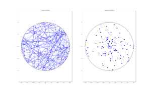
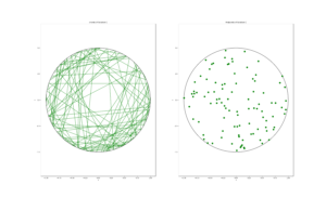
Simulating a Poisson point process on a disk
Simulating a Poisson point process on a triangle
Simulating an inhomogeneous Poisson point process
Simulating a Matérn cluster point process
Simulating a Thomas cluster point process
The Julia code, like all the code I present here, can be found on my Github repository, which for this post is located here.
Basics
Language type and syntax
The Wikipedia article on Julia says:
Julia is a high-level general-purpose dynamic programming language designed for high-performance numerical analysis and computational science.
Scientific programming languages like the popular three MATLAB, R and Python, are interpreted languages. But the people behind Julia say:
it is a flexible dynamic language, appropriate for scientific and numerical computing, with performance comparable to traditional statically-typed languages.
Because Julia’s compiler is different from the interpreters used for languages like Python or R, you may find that Julia’s performance is unintuitive at first.
I already remarked that Julia’s syntax is clearly inspired by MATLAB, as one can see in this guide for MATLAB, Python and Julia. But there are key differences. For example, to access an array entry in Julia, you use square brackets (like in most programming languages), whereas parentheses are used in MATLAB or, that old mathematical programming classic, Fortran, which is not a coincidence.
Packages
Julia requires you to install certain packages or libraries, like most languages. For random simulations and plots, you have to install the respective Julia packages Distributions and Plots, which is done by running the code.
Pkg.add("Distributions");
Pkg.add("Plots");
After doing that, it’s best to restart Julia. These packages are loaded with the using command:
Using Distributions;
Using Plots;
Also, the first time it takes a while to run any code using those newly installed packages.
I should stress that there are different plotting libraries. But Plots, which contains many plotting libraries, is the only one I could get working. Another is PlotPy, which uses the Python library. As a beginner, it seems to me that the Julia community has not focused too much on developing new plotting functions, and has instead leveraged pre-existing libraries.
For standard scientific and statistical programming, you will usually also need the packages LinearAlgebra and Statistics.
Data types
Unlike MATLAB or R, Julia is a language that has different data types for numbers, such as integers and floating-point numbers (or floats). This puts Julia in agreement with the clear majority of languages, making it nothing new for most programmers. This is not a criticism of the language, but this can be troublesome if you’ve grown lazy after years of using MATLAB and R.
Simulating random variables
In MATLAB, R and Python, we just need to call a function for simulating uniform, Poisson, and other random variables. There’s usually a function for each type of random variable (or probability distribution).
Julia does simulation of random objects in a more, let’s say, object-oriented way (but I’m told, it’s not an object-oriented language). The probability distributions of random variables are objects, which are created and then sent to a general function for random generation. For example, here’s the code for simulating a Poisson variable with mean \(\mu=10\).
mu=10;
distPoisson=Poisson(mu);
numbPoisson=rand(distPoisson);
Similarly, here’s how to simulate a normal variable with mean \(\mu=10\) and standard deviation \(\sigma=1\).
mu=10;
sigma=1;
distNormal=Normal(mu,sigma);
numbNormal=rand(distNormal);
Of course the last two lines can be collapsed into one.
mu=10;
sigma=1;
numbNormal=rand(Normal(mu,sigma));
But if you just want to create standard uniform variables on the interval (0,1), then the code is like that in MATLAB. For example, this code creates a \(4\times3\) matrix (or array) \(X\) whose entries are simulation outcomes of independent uniform random variables:
X=rand(4,3);
The resulting matrix \(X\) is a Float 64 array.
Arrays
The indexing of arrays in Julia starts at one, just like MATLAB, R, or Fortran. When you apply a function to an array, you generally need to use the dot notation. For example, if I try to run the code:
Y=sqrt(rand(10,1)); #This line will result in an error.
then on my machine (with Julia Version 1.0.3) I get the error:
ERROR: DimensionMismatch(“matrix is not square: dimensions are (10, 1)”)
But this code works:
Y=sqrt.(rand(10,1));
Also, adding scalars to arrays can catch you in Julia, as you also often need to use the dot notation. This code:
Y=sqrt.(rand(10,1));
Z=Y+1; #This line will result in an error.
gives the error:
ERROR: MethodError: no method matching +(::Array{Float64,2}, ::Int64)
This is fixed by adding a dot:
Y=sqrt.(rand(10,1));
Z=Y.+1; #This line will work.
Note the dot has to be on the left hand side. I ended up just using dot notation every time to be safe.
Other traps exist. For example, with indexing, you need to convert floats to integers if you want to use them as indices.
Repeating array elements
There used to be a Julia function called repmat, like the one in MATLAB , but it was merged with a function called repeat. I used such repeating operations to avoid explicit for-loops, which is generally advised in languages like MATLAB and R. For example, I used the repelem function in MATLAB to simulate Matérn and Thomas cluster point processes. To do this in Julia, I had to use this nested construction:
y=vcat(fill.(x, n)...);
This line means that the first value in \(x \) is repeated \(n[1]\) times, where \(n[1]\) is the first entry of \(n\) (as indexing in Julia starts at one), then the second value of \(x\) is repeated \(n[2]\) times, and so on. For example, the vectors \(x=[7,4,9]\) and \(n=[2,1,3]\), the answer is \(y=[7,7,4,9,9,9]\).
To do this in Julia, the construction is not so bad, if you know how, but it’s not entirely obvious. In MATLAB I use this:
y=repelem(x,n);
Similarly in Python:
y=np.repeat(x,n);
Different versions of Julia
I found that certain code would work (or not work) and then later the same code would not work (or would work) on machines with different versions of Julia, demonstrating how the language is still being developed. More specifically, I ran code on Julia Version 1.0.3 (Date 2018-12-18) and Julia Version 0.6.4 (Date: 2018-07-09). (Note how there’s only a few months difference in the dates of the two versions.)
Consider the code with the errors (due to the lack of dot operator) in the previous section. The errors occurred on one machine with Julia Version 1.0.3, but the errors didn’t occur on another machine with the older Julia Version 0.6.4. For a specific example, the code:
Y=sqrt.(rand(10,1));
Z=Y+1; #This line will not result in an error on Version 0.6.4.
gives no error with Julia Version 0.6.4, while I have already discussed how it gives an error with Julia Version 1.0.3.
For another example, I copied from this MATLAB-Python-Julia guide the following command:
A = Diagonal([1,2,3]); #This line will (sometimes?) result in an error.
It runs on machine with Julia Version 0.6.4 with no problems. But running it on the machine with Julia Version 1.0.3 gives the error:
ERROR: UndefVarError: Diagonal not defined
That’s because I have not used the LinearAlgebra package. Fixing this, the following code:
using LinearAlgebra; #Package needed for Diagonal command.
A = Diagonal([1,2,3]); #This line should now work.
gives no error with Julia Version 1.0.3.
If you have the time and energy, you can search the internet and find online forums where the Julia developers have discussed why they have changed something, rendering certain code unworkable with the latest versions of Julia.
Optimization
It seems that performing optimization on functions is done with the Optim package.
Pkg.add("Optim");
But some functions need the Linesearches package, so it’s best to install that as well.
Pkg.add("Linesearches");
Despite those two optimization packages, I ended up using yet another package called BlackBoxOptim.
Pkg.add("BlackBoxOptim");
In this package, I used a function called bboptimize. This is the first optimziation function that I managed to get working. I do not know how it compares to the functions in the Optim and Linesearches packages.
In a previous post, I used optimization functions to simulate a inhomogeneous or nonhomogeneous Poisson point process on a rectangle. I’ve also written Julia code for this simulation, which is found below. I used bboptimize, but I had some problems when I initially set the search regions to integers, which the package did not like, as the values need to be floats. That’s why I multiple the rectangle dimensions by \(1.0\) in the following code:
boundSearch=[(1.0xMin,1.0xMax), (1.0yMin, 1.0yMax)]; #bounds for search box
#WARNING: Values of boundSearch cannot be integers!
resultsOpt=bboptimize(fun_Neg;SearchRange = boundSearch);
lambdaNegMin=best_fitness(resultsOpt); #retrieve minimum value found by bboptimize
Conclusion
In this brief experiment, I found the language Julia good for doing stochastic simulations, but too tricky for doing simple things like plotting. Also, depending on the version of Julia, sometimes my code would work and sometimes it wouldn’t. No doubt things will get better with time.
Further reading
As I said, Julia is still very much an ongoing project. Here’s a couple of links that helped me learn the basics.
https://en.wikibooks.org/wiki/Introducing_Julia/Arrays_and_tuples
https://voxeu.org/content/which-numerical-computing-language-best-julia-matlab-python-or-r
Julia, Matlab, and C
https://modelingguru.nasa.gov/docs/DOC-2676
Code
I’ve only posted here code for some of simulations, but the rest of the code is available on my GitHub repository located here. You can see how the code is comparable to that of MATLAB.
Poisson point process on a rectangle
I wrote about this point process here. The code is located here.
using Distributions #for random simulations
using Plots #for plotting

#Simulation window parameters
xMin=0;xMax=1;
yMin=0;yMax=1;
xDelta=xMax-xMin;yDelta=yMax-yMin; #rectangle dimensions
areaTotal=xDelta*yDelta;

#Point process parameters
lambda=100; #intensity (ie mean density) of the Poisson process

#Simulate Poisson point process
numbPoints=rand(Poisson(areaTotal*lambda)); #Poisson number of points
xx=xDelta*rand(numbPoints,1).+xMin;#x coordinates of Poisson points
yy=yDelta*(rand(numbPoints,1)).+yMin;#y coordinates of Poisson points

#Plotting
plot1=scatter(xx,yy,xlabel ="x",ylabel ="y", leg=false);
display(plot1);
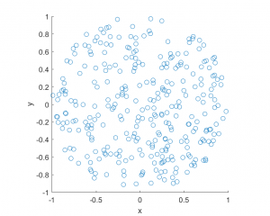
Inhomogeneous Poisson point process on a rectangle
I wrote about this point process here. The code is located here.
using Distributions #for random simulations
using Plots #for plotting
using BlackBoxOptim #for blackbox optimizing

#Simulation window parameters
xMin=-1;xMax=1;
yMin=-1;yMax=1;
xDelta=xMax-xMin;yDelta=yMax-yMin; #rectangle dimensions
areaTotal=xDelta*yDelta;

s=0.5; #scale parameter

#Point process parameters
function fun_lambda(x,y)
    100*exp.(-(x.^2+y.^2)/s^2); #intensity function
end

###START -- find maximum lambda -- START ###
#For an intensity function lambda, given by function fun_lambda,
#finds the maximum of lambda in a rectangular region given by
#[xMin,xMax,yMin,yMax].
#NOTE: Need xMin, xMax, yMin, yMax to be floats eg xMax=1. See boundSearch

function fun_Neg(x)
     -fun_lambda(x[1],x[2]); #negative of lambda
end
xy0=[(xMin+xMax)/2.0,(yMin+yMax)/2.0];#initial value(ie centre)

#Find largest lambda value
boundSearch=[(1.0xMin,1.0xMax), (1.0yMin, 1.0yMax)];
#WARNING: Values of boundSearch cannot be integers!
resultsOpt=bboptimize(fun_Neg;SearchRange = boundSearch);
lambdaNegMin=best_fitness(resultsOpt); #retrieve minimum value found by bboptimize
lambdaMax=-lambdaNegMin;
###END -- find maximum lambda -- END ###

#define thinning probability function
function fun_p(x,y)
    fun_lambda(x,y)/lambdaMax;
end

#Simulate a Poisson point process
numbPoints=rand(Poisson(areaTotal*lambdaMax)); #Poisson number of points
xx=xDelta*rand(numbPoints,1).+xMin;#x coordinates of Poisson points
yy=yDelta*(rand(numbPoints,1)).+yMin;#y coordinates of Poisson points

#calculate spatially-dependent thinning probabilities
p=fun_p(xx,yy);
#Generate Bernoulli variables (ie coin flips) for thinning
booleRetained=rand(numbPoints,1).<p; #points to be retained
xxRetained=xx[booleRetained]; yyRetained=yy[booleRetained];

#Plotting
plot1=scatter(xxRetained,yyRetained,xlabel ="x",ylabel ="y", leg=false);
display(plot1);
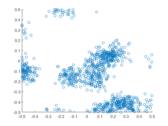
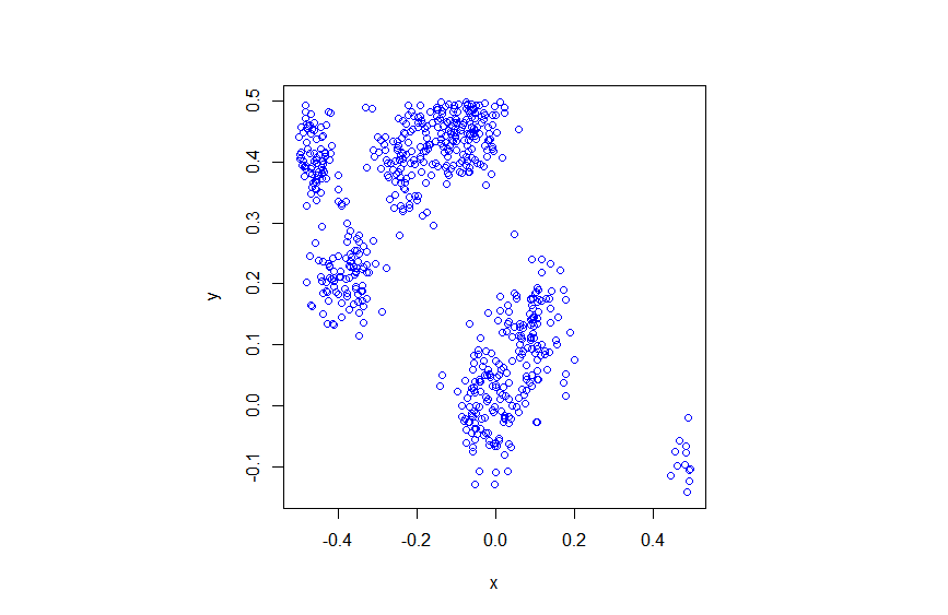
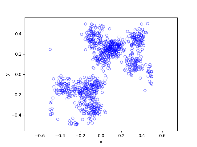
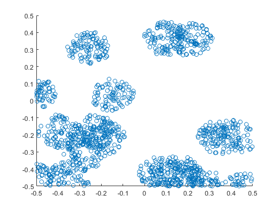
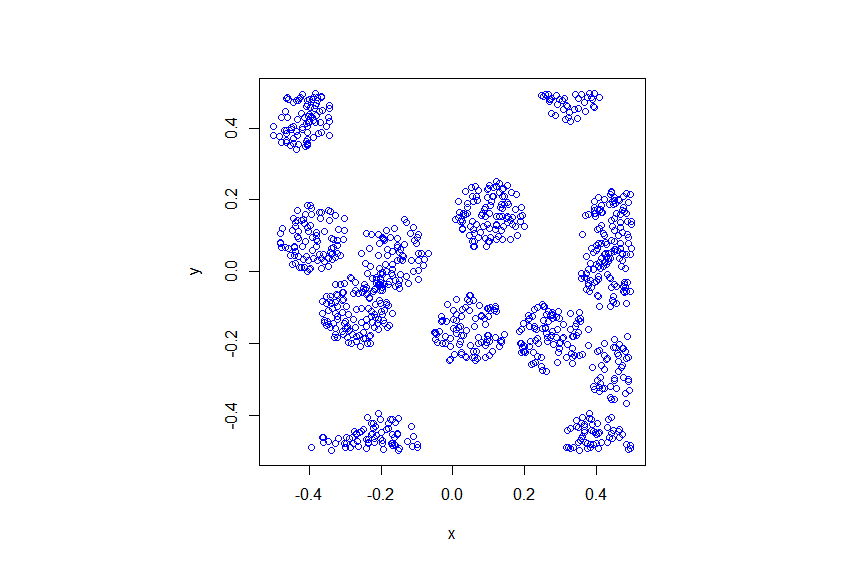
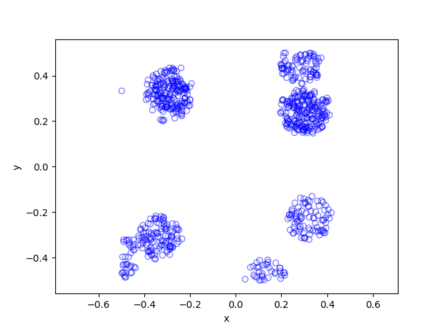
Thomas point process on a rectangle
I wrote about this point process here. The code is located here.
using Distributions #for random simulations
using Plots #for plotting

#Simulation window parameters
xMin=-.5;
xMax=.5;
yMin=-.5;
yMax=.5;

#Parameters for the parent and daughter point processes
lambdaParent=10;#density of parent Poisson point process
lambdaDaughter=10;#mean number of points in each cluster
sigma=0.05; #sigma for normal variables (ie random locations) of daughters

#Extended simulation windows parameters
rExt=7*sigma; #extension parameter
#for rExt, use factor of deviation sigma eg 6 or 7
xMinExt=xMin-rExt;
xMaxExt=xMax+rExt;
yMinExt=yMin-rExt;
yMaxExt=yMax+rExt;
#rectangle dimensions
xDeltaExt=xMaxExt-xMinExt;
yDeltaExt=yMaxExt-yMinExt;
areaTotalExt=xDeltaExt*yDeltaExt; #area of extended rectangle

#Simulate Poisson point process
numbPointsParent=rand(Poisson(areaTotalExt*lambdaParent)); #Poisson number of points

#x and y coordinates of Poisson points for the parent
xxParent=xMinExt.+xDeltaExt*rand(numbPointsParent,1);
yyParent=yMinExt.+yDeltaExt*rand(numbPointsParent,1);

#Simulate Poisson point process for the daughters (ie final poiint process)
numbPointsDaughter=rand(Poisson(lambdaDaughter),numbPointsParent);
numbPoints=sum(numbPointsDaughter); #total number of points

#Generate the (relative) locations in Cartesian coordinates by
#simulating independent normal variables
xx0=rand(Normal(0,sigma),numbPoints);
yy0=rand(Normal(0,sigma),numbPoints);

#replicate parent points (ie centres of disks/clusters)
xx=vcat(fill.(xxParent, numbPointsDaughter)...);
yy=vcat(fill.(yyParent, numbPointsDaughter)...);

#Shift centre of disk to (xx0,yy0)
xx=xx.+xx0;
yy=yy.+yy0;

#thin points if outside the simulation window
booleInside=((xx.>=xMin).&(xx.<=xMax).&(yy.>=yMin).&(yy.<=yMax));
#retain points inside simulation window
xx=xx[booleInside];
yy=yy[booleInside];

#Plotting
plot1=scatter(xx,yy,xlabel ="x",ylabel ="y", leg=false);
display(plot1);