Poisson (stochastic) process

One of the most important stochastic processes is Poisson stochastic process, often called simply the Poisson process. In a previous post I gave the definition of a stochastic process (also called a random process) alongside some examples of this important random object, including counting processes.  The Poisson (stochastic) process is a counting process. This continuous-time  stochastic process is a highly studied and used object. It plays a key role in different probability fields, particularly those focused on stochastic processes such as stochastic calculus (with jumps) and the theories of Markov processes, queueingpoint processes (on the real line), and Levy processes.

The points in time when a Poisson stochastic process increases form a Poisson point process on the real line. In this setting the stochastic process and the point process can be considered two interpretations of the same random object.  The Poisson point process is often just called the Poisson process, but a Poisson point process can be defined on more generals spaces. In some literature, such as the theory of Lévy processes, a Poisson point process is called a Poisson random measure, differentiating the Poisson point process from the Poisson stochastic process. Due to the connection with the Poisson distribution, the two mathematical objects are named after Simeon Poisson, but he never studied these random objects.

The other important stochastic process is the Wiener process or Brownian (motion process), which I cover in another post. The Wiener process is arguably the most important stochastic process. I have written that post and the current one with the same structure and style, reflecting and emphasizing the similarities between these two fundamental stochastic process.

In this post I will give a definition of the homogenous Poisson process. I will also describe some of its key properties and importance. In future posts I will cover the history and generalizations of this stochastic process.

Definition

In the stochastic processes literature there are different definitions of the Poisson process. These depend on the settings such as the level of mathematical rigour. I give a mathematical definition which captures the main characteristics of this stochastic process.

Definition: Homogeneous Poisson (stochastic) process

An integer-valued stochastic process \(\{N_t:t\geq 0 \}\) defined on a probability space \((\Omega,\mathcal{A},\mathbb{P})\) is a homogeneous Poisson (stochastic) process if it has the following properties:

  1. The initial value of the stochastic process \(\{N_t:t\geq 0 \}\) is zero with probability one, meaning \(P(N_0=0)=1\).
  2. The increment \(N_t-N_s\) is independent of the past, that is, \(N_u\), where \(0\leq u\leq s\).
  3. The increment \(N_t-N_s\) is a Poisson variable with mean \(\lambda (t-s)\).

In some literature, the initial value of the stochastic process may not be given. Alternatively, it is simply stated as \(N_0=0\) instead of the more precise (probabilistic) statement given above.

Also, some definitions of this stochastic process include an extra property or two. For example, from the above definition, we can infer that increments of the homogeneous Poisson process are stationary due to the properties of the Poisson distribution. But a definition may include something like the following property, which explicitly states that this stochastic process is stationary.

  1. For \(0\leq u\leq s\), the increment \(N_t-N_s\) is equal in distribution to \(N_{t-s}\).

The definitions may also describe the continuity of the realizations of the stochastic process, known as sample paths, which we will cover in the next section.

It’s interesting to compare these defining properties with the corresponding ones of the standard Wiener stochastic process. Both stochastic processes build upon divisible probability distributions. Using this property, Lévy processes generalize these two stochastic processes.

Properties

The definition of the Poisson (stochastic) process means that it has stationary and independent increments. These are arguably the most important properties as they lead to the great tractability of this stochastic process. The increments are Poisson random variables, implying they can have only positive (integer) values.

The Poisson (stochastic) process exhibits closure properties, meaning you apply certain operations, you get another Poisson (stochastic) process. For example, if we sum two independent Poisson processes \(X= \{X_t:t\geq 0 \}\) and \(Y= \{Y_t:t\geq 0 \}\), then the resulting stochastic process \(Z=Z+Y = \{N_t:t\geq 0 \}\) is also a Poisson (stochastic) process. Such properties are useful for proving mathematical results.

A single realization of a (homogeneous) Poisson stochastic process, where the blue marks show where the process jumps to the next value. In any finite time interval, there are a finite number of jumps.

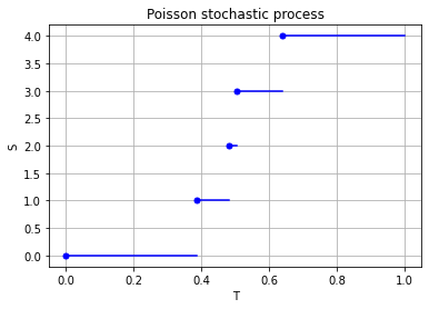
Properties such as independence and stationarity of the increments are so-called distributional properties. But the sample paths of this stochastic process are also interesting. A sample path of a Poisson stochastic process is  almost surely non-decreasing, being constant except for jumps of size one. (The term almost surely comes from measure theory, but it means with probability one.) There are only finitely number of jumps in each finite time interval.

The homogeneous Poisson (stochastic) process has the Markov property, making it an example of a Markov process.  The homogenous Poisson process \(N=\{ N_t\}_{t\geq 0}\)s not a martingale. But interestingly, the stochastic process is \(\{ W_t – \lambda t\}_{t\geq 0}\) is a martingale. (Such relations have been used to study such stochastic processes with tools from martingale theory.)

Stochastic or point process?

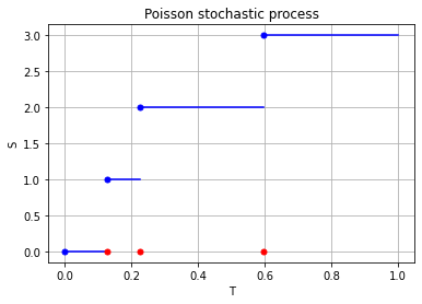
The Poisson (stochastic) process is a discrete-valued stochastic process in continuous time. The relation these types of stochastic processes and point process is a subtle one. For example, David Cox and Valerie Isham write on page 3 of their monograph:

 The borderline between point processes and a  number of other kinds of stochastic process is not sharply defined. In particular, any stochastic process in continuous time in which the sample paths are step functions, and therefore any any process with a discrete state space, is associated with a point process, where a point is a time of transition or, more generally, a time of entry into a pre-assigned state or set of states. Whether it is useful to look at a particular process in this way depends on the purpose of the analysis.

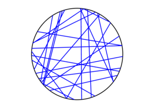
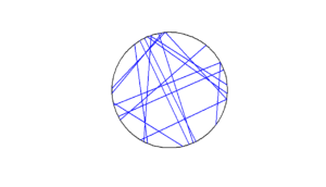
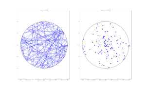
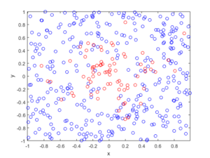
For the Poisson case, this association is presented in the diagram below. We can see the Poisson point process (in red) associated with the Poisson (stochastic) process (in blue) by simply looking at the time points where jumps occur.

A single realization of a (homogeneous) Poisson stochastic process (in blue). The jumps of the process form a (homogeneous) Poisson point process (in red) on the real line representing time.

Importance

Playing a prominent role in the theory of probability, the Poisson (stochastic) process is a highly important and studied stochastic process. It has connections to other stochastic processes and is central in queueing theory and random measures.

The Poisson process is a building block for more complex continuous-time Markov processes with discrete state spaces, which are used as mathematical models.  It is also essential in the study of jump processes and subordinators.

The Poisson (stochastic) process is a member of some important families of stochastic processes, including Markov processes, Lévy processes, and birth-death processes. This stochastic process also has many applications. For example, it plays a central role in quantitative finance. It is also used in the physical sciences as well as some branches of social sciences, as a mathematical model for various random phenomena.

Generalizations and modifications

For the Poisson (stochastic) process, the index set and state space are respectively the non-negative numbers and counting numbers, that is \(T=[0,\infty)\) and \(S=0, 1, \dots\), so it has a continuous index set but a discrete state space. Consequently, changing the state space, index set, or both offers an ways for generalizing and modifying the Poisson (stochastic) process.

Simulation

The defining properties of the Poisson stochastic process, namely independence and stationarity of increments, results in it being easy to simulate. The Poisson  stochastic process can be simulated provided random variables can be simulated or sampled according to a Poisson distributions, which I have covered in this and this post.

Simulating a Poisson stochastic process is similar to simulating a Poisson point process. (Basically, it is the same method in a one-dimensional setting.) But I will leave the details of sampling this stochastic process for another post.

Further reading

Here are some related links:

A very quick history of Wiener process and the Poisson (point and stochastic) process is covered in this talk by me.

In terms of books, the Poisson process has not received as much attention as the Wiener process, which is typically just called the Brownian (motion) process.  That said, any book covering queueing theory will cover the Poisson (stochastic) process.

More advanced readers can read about the Poisson (stochastic) process, the Wiener (or Brownian (motion)) process, and other Lévy processes:

On this topic, I recommend the introductory article:

  • 2004, Applebaum, Lévy Processes – From Probability to Finance and Quantum Groups.

This stochastic process is of course also covered in general books on stochastics process such as:


Summary: Poisson simulations

Here’s a lazy summary post where I list all the posts on various Poisson simulations. I’ve also linked to code, which is found on this online repository. The code is typically written in MATLAB and Python.

Posts

Poisson point processes

Some simulations of Poisson point processes are also covered in this post on the Julia programming language:

Checking simulations

Poisson line process

Poisson random variables

Simulating a Poisson point process on a n-dimensional sphere

In the previous post I outlined how to simulate or sample a homogeneous Poisson point process on the surface of a sphere. Now I will consider a homogeneous Poisson point process on the \((n-1)-\) sphere, which is the surface of the Euclidean ball in \(n\) dimensions.

This is a short post because it immediately builds off the previous post. For positioning the points uniformly, I will use Method 2 from that post, which uses normal random variables, as it immediately gives a fast method in \(n\) dimensions.

I wrote this post and the code more for curiosity than any immediate application. But simulating a Poisson point process in this setting requires placing points uniformly on a sphere. And there are applications in that, such as Monte Carlo integration methods, as mentioned in this post, which nicely details different sampling methods.

Steps

As is the case for other shapes, simulating a Poisson point process requires two steps.

Number of points

The number of points of a Poisson point process on the surface of a sphere of radius \(r>0\) is a Poisson random variable. The mean of this random variable is \(\lambda S_{n-1}\), where \(S_{n-1}\) is the surface area of the sphere.  For a ball embedded in \(n\) dimension, the area of the corresponding sphere is given by

$$S_{n-1} = \frac{2 \pi ^{n/2}  }{\Gamma(n/2)} r^{n-1},$$

where \(\Gamma\) is the gamma function, which is a natural generalization of the factorial. In MATLAB, we can simply use the function gamma.  In Python, we need to use the SciPy function scipy.special. gamma.

Locations of points

For each point on the sphere, we generate \(n\) standard normal or Gaussian random variables, say, \(W_1, \dots, W_n\), which are independent of each other. These random variables are the Cartesian components of the random point. We rescale the components by the Euclidean norm, then multiply by the radius \(r\).

For \(i=1,\dots, n\), we obtain

$$X_i=\frac{rW_i}{(W_1^2+\cdots+W_n^2)^{1/2}}.$$

These are the Cartesian coordinates of a point uniformly scattered on a  sphere with radius \(r\) and a centre at the origin.

How does it work?

In the post on the circle setting, I gave a more detailed outline of the proof, where I said the method is like the Box-Muller transform in reverse. The joint density of the normal random variables is from a multivariate normal distribution with zero correlation. This joint density a function of the Cartesian equation for a sphere. This means the density is constant on the sphere, implying that the angle of the point \((W_1,\dots, W_n)\) will be uniformly distributed.

The vector formed from the normal variables \((W_1,\dots,W_n)\) is a random variable with a chi distribution.  But the final vector, which stretches from the origin to the point \((X_1,\dots,X_n)\), has length one, because we rescaled it with the Euclidean norm.

Code

The code for all my posts is located online here. For this post, the code in MATLAB and Python is here.

Further reading

I recommend this blog post, which discusses different methods for randomly placing points on spheres and inside spheres (or, rather, balls) in a uniform manner.  (Embedded in two dimensions, a sphere is a circle and a ball is a disk.)

Our Method 2 for positioning points uniformly, which uses normal variables, comes from the paper:

  • 1959, Muller, A note on a method for generating points uniformly on n-dimensional spheres.

Two recent works on this approach are the papers:

  • 2010, Harman and Lacko, On decompositional algorithms for uniform sampling from -spheres and -balls;
  • 2017, Voelker, Gosman, Stewart, Efficiently sampling vectors and coordinates.

Simulating a Poisson point process on a sphere

In this post I’ll describe how to simulate or sample a homogeneous Poisson point process on the surface of a sphere. I have already simulated this point process on a rectangle, triangle disk, and circle.

Of course, by sphere, I mean the everyday object that is the surface of a three-dimensional ball, where this two-dimensional object is often denoted by \(S^2\).  Mathematically, this is a generalization from a Poisson point process on a circle, which is slightly simpler than randomly positioning points on a disk.  I recommend reading those two posts first, as a lot of the material presented here builds off them.

I have not needed such a simulation in my own work, but I imagine there are many reasons why you would want to simulate a Poisson point process on a sphere. As some motivation, we can imagine these points on a sphere representing, say, meteorites or lightning hitting the Earth.

The generating the number of points is not difficult. The trick is positioning the points on the sphere in a uniform way.  As is often the case, there are various ways to do this, and I recommend this post, which lists the main ones.  I will use two methods that I consider the most natural and intuitive ones, namely using spherical coordinates and normal random variables, which is what I did in the post on the circle.

Incidentally, a simple modification allows you to scatter the points uniformly inside the sphere, but you would typically say ball in mathematics, giving a Poisson point process inside a ball; see below for details.

Steps

As always, simulating a Poisson point process requires two steps.

Number of points

The number of points of a Poisson point process on the surface of a sphere of radius \(r>0\) is a Poisson random variable with mean \(\lambda S_2\), where \(S_2=4\pi r^2\) is the surface area of the sphere. (In this post I give some details for simulating or sampling Poisson random variables or, more accurately, variates.)

Locations of points

For any homogeneous Poisson point process, we need to position the points uniformly on the underlying space, which is in this case is the sphere. I will outline two different methods for positioning the points randomly and uniformly on a sphere.

Method 1: Spherical coordinates

The first method is based on spherical coordinates \((\rho, \theta,\phi)\), where the radial coordinate \(\rho\geq 0\), and the angular coordinates \(0 \leq \theta\leq 2\pi\) and \(0\leq \phi \leq \pi\). The change of coordinates gives \(x=\rho\sin(\theta)\cos(\phi)\), \(y=\rho\sin(\theta)\sin(\phi)\), and \(z=\rho\cos(\phi)\).

Now we use Proposition 1.1 in this paper. For each point, we generate two uniform variables \(V\) and \(\Theta\) on the respective intervals \((-1,1)\) and \((0,2\pi)\). Then we place the point with the Cartesian coordinates

$$X =  r  \sqrt{1-V^2} \cos\Theta, $$

$$Y =  r  \sqrt{1-V^2}\sin\Theta, $$

$$ Z=r V. $$

This method places a uniform point on a sphere with a radius \(r\).

How does it work?

I’ll skip the precise details, but give some interpretation of this method. The random variable \(\Phi := \arccos V\) is the \(\phi\)-coordinate of the uniform point, which implies \(\sin \Phi=\sqrt{1-V^2}\), due to basic trigonometric identities.  The area element in polar coordinates is \(dA = \rho^2 \sin\phi d\phi d\theta \), which is constant with respect to \(\theta\). After integrating with respect to \(\phi\),  we see that the random variable \(V=\cos\Phi\) needs to be uniform (instead of \(\Phi\)) to ensure the point is uniformly located on the surface.

Method 2: Normal random variables

For each point, we generate three standard normal or Gaussian random variables, say, \(W_x\), \(W_y\), and \(W_z\), which are independent of each other. (The term standard here means the normal random variables have mean \(\mu =0\) and standard deviation \(\sigma=1\).)  The three random variables are the Cartesian components of the random point. We rescale the components by the Euclidean norm, then multiply by the radius \(r\), giving

$$X=\frac{rW_x}{(W_x^2+W_y^2+W_z^2)^{1/2}},$$

$$Y=\frac{rW_y}{(W_x^2+W_y^2+W_z^2)^{1/2}},$$

$$Z=\frac{rW_z}{(W_x^2+W_y^2+W_z^2)^{1/2}}.$$

These are the Cartesian coordinates of a point uniformly scattered on a  sphere with radius \(r\) and a centre at the origin.

How does it work?

The procedure is somewhat like the Box-Muller transform in reverse. In the post on the circle setting,  I gave an outline of the proof, which I recommend reading. The joint density of the normal random variables is from a multivariate normal distribution with zero correlation. This joint density is constant on the sphere, implying that the angle of the point \((W_x, W_y, W_z)\) will be uniformly distributed.

The vector formed from the normal variables \((W_x, W_y,W_z)\) is a random variable with a chi distribution.  We can see that the vector from the origin to the point \((X,Y,Z)\) has length one, because we rescaled it with the Euclidean norm.

Plotting

Depending on your plotting software, the points may more resemble points on an ellipsoid than a sphere due to the different scaling of the x, y and z axes. To fix this in MATLAB, run the command: axis square. In Python, it’s not straightforward to do this, as it seems to lack an automatic function, so I have skipped it.

Results

I have presented some results produced by code written in MATLAB and Python. The blue points are the Poisson points on the sphere. I have used a surface plot (with clear faces) to illustrate the underling sphere in black.

MATLAB

Python

Note: The aspect ratio in 3-D Python plots tends to squash the sphere slightly, but it is a sphere.

Code

The code for all my posts is located online here. For this post, the code in MATLAB and Python is here.  In Python I used the library mpl_toolkits for doing 3-D plots.

Poisson point process inside the sphere

Perhaps you want to simulate a Poisson point process inside the ball.  There are different ways we can do this, but I will describe just one way, which builds off Method 1 for positioning the points uniformly. (In a later post, I will modify Method 2, giving a way to uniformly position points inside the ball.)

For this simulation method, you need to make two simple modifications to the simulation procedure.

Number of points

The number of points of a Poisson point process inside a sphere of radius \(r>0\) is a Poisson random variable with mean \(\lambda V_3\), where \(V_3=4\pi r^3\) is the volume of the sphere.

Locations of points

We will modify Method 1 as outlined above. To sample the points uniformly in the sphere, you need to generate uniform variables on the unit interval \((0,1)\), take their cubic roots, and then, multiply them by the radius \(r\). (This is akin to the step of taking the square root in the disk setting.) The random variables for the angular coordinates are generated as before.

Further reading

I recommend this blog post, which discusses different methods for randomly placing points on spheres and inside spheres (or, rather, balls) in a uniform manner.  (Embedded in two dimensions, a sphere is a circle and a ball is a disk.)

Our Method 2 for positioning points uniformly, which uses normal variables, comes from the paper:

  • 1959, Muller, A note on a method for generating points uniformly on n-dimensional spheres.

This sampling method relies upon old observations that normal variables are connected to spheres and circles. I also found this post on a similar topic. Perhaps not surprisingly, the above paper is written by the same Muller behind the Box-Muller method for sampling normal random variables.

Update: The connection between the normal distribution and rotational symmetry has been the subject of some recent 3Blue1Brown videos on YouTube.

Here is some sample Python code for creating a 3-D scatter plot.

Signal strengths of a wireless network

In two previous posts, here and here, I discussed the importance of the quantity called the signal-to-interference ratio, which is usually abbreviated as SIR, for studying communication in wireless networks. In everyday terms, for a listener to hear a certain speaker in a room full of people speaking, the ratio of the speaker’s volume to the sum of the volumes of everyone else heard by the listener. The SIR is the communication bottleneck for any receiver and transmitter pair in a wireless network.

But the strengths (or power values) of the signals are of course also important. In this post I will detail how we can model them using a a simple network model with a single observer.

Propagation model

For a transmitter located at \(X_i\in \mathbb{R}^2\), researchers usually attempt to represent the received power of the signal \(P_i\) with a propagation model. Assuming the power is received at \(x\in \mathbb{R}^2\), this mathematical model consists of a random and a deterministic component taking the general form
$$
P_i(x)=F_i\,\ell(|X_i-x|) ,
$$
where \(\ell(r)\) is a non-negative function in \(r>0\) and \(F_i\) is a non-negative random variable.

The function \(\ell(r)\) is called the pathloss function, and common choices include \(\ell(r)=(\kappa r)^{-\beta}\) and \(\ell(r)=\kappa e^{-\beta r}\), where \(\beta>0\) and \(\kappa>0\) are model constants.

The random variables \(F_i\) represent signal phenomena such as multi-path fading and shadowing (also called shadow fading), caused by the signal interacting with the physical environment such as buildings. It is often called fading or shadowing variables.

We assume the transmitters locations \(X_1,\dots,X_n\) are on the plane \(\mathbb{R}^2\). Researchers typically assume they form a random point process or, more precisely, the realization of a random point process.

From two dimensions to one dimension

For studying wireless networks, a popular technique is to consider a wireless network from the perspective of a single observer or user. Researchers then consider the incoming or received signals from the entire network at the location of this observer or user. They do this by considering the inverses of the signal strengths, namely

$$
L_i(x): = \frac{1}{P_i}=\frac{1}{F_i \,\ell(|X_i-x|) }.
$$

Mathematically, this random function is simply a mapping from the two-dimensional plane \(\mathbb{R}^2\) to the one-dimensional non-negative real line \(\mathbb{R}_0^+=[0,\infty)\).

If the transmitters are located according to a non-random point pattern or a random point process, this random mapping generates a random point process on the non-negative real line. The resulting one-dimensional point process of the values \(L_1,L_2,\dots, \) has been called (independently) propagation (loss) process or path loss (with fading) process. More recently, my co-authors and I decided to call it a projection process, but of course the precise name doesn’t mattter

Intensity measure of signal strengths

Assuming a continuous monotonic path loss function \(\ell\) and the fading variables \(F_1, F_2\dots\) are iid, if the transmitters form a stationary random point process with intensity \(\lambda\), then the inverse signal strengths \(L_1,L_2,\dots \) form a random point process on the non-negative real line with the intensity measure \(M\).

$$
M(t) =\lambda \pi \mathbb{E}( [\ell(t F)^{-1} ]^2)\,,
$$

where \(\ell^{-1}\) is the generalized inverse of the function \(\ell\). This expression can be generalized for a non-stationary point process with general intensity measure \(\Lambda\).

The inverses \(1/L_1,1/L_2,\dots \), which are the signal strengths, forprocess with intensity measure

$$
\bar{M}(s) =\lambda \pi \mathbb{E}( [\ell( F/s)^{-1} ]^2).
$$

Poisson transmitters gives Poisson signal strengths

Assuming a continuous monotonic path loss function \(\ell\) and the fading variables \(F_1, F_2\dots\) are iid, if the transmitters form a Poisson point process with intensity \(\lambda\), then the inverse signal strengths \(L_1,L_2,\dots \) form a Poisson point process on the non-negative real line with the intensity measure \(M\).

If \(L_1,L_2,\dots \) form a homogeneous Poisson point process, then the inverses \(1/L_1,1/L_2,\dots \) will also form a Poisson point process with intensity measure \(\bar{M}(s) =\lambda \pi \mathbb{E}( [\ell( F/s)^{-1} ]^2). \)

Propagation invariance

For \(\ell(r)=(\kappa r)^{-\beta}\) , the expression for the intensity measure \(M\) reduces to
$$
M(t) = \lambda \pi t^{-2/\beta} \mathbb{E}( F^{-2/\beta})/\kappa^2.
$$

What’s striking here is that information of the fading variable \(F\) is captured simply by one moment \(\mathbb{E}( F^{-2/\beta}) \). This means that two different distributions will give the same results as long as this moment is matching. My co-authors and I have been called this observation propagation invariance.

Some history

To study just the (inverse) signal strengths as a point process on the non-negative real line was a very useful insight. It was made independently in these two papers:

  • 2008, Haenggi, A geometric interpretation of fading in wireless
    networks: Theory and applications;
  • 2010, Błaszczyszyn, Karray, and Klepper, Impact of the geometry, path-loss exponent and random shadowing on the mean interference factor in wireless cellular networks.

My co-authors and I presented a general expression for the intensity measure \(M\) in the paper:

  • 2018, Keeler, Ross and Xia, When do wireless network signals appear Poisson?.

This paper is also contains examples of various network models.

Further reading

A good starting point on this topic is the Wikipedia article Stochastic geometry models of wireless networks. The paper that my co-authors and I wrote has details on the projection process.

With Bartek Błaszczyszyn, Sayan Mukherjee, and Martin Haenggi, I co-wrote a short monograph on SINR models called Stochastic Geometry Analysis of Cellular Networks, which is written at a slightly more advanced level. The book puts an emphasis on studying the point process formed from inverse signal strengths, we call the projection process.

Simulating a Poisson line process

Instead of points, we can consider other objects randomly scattered on some underlying mathematical space. If we take a Poisson point process, then we can use (infinitely long) straight lines instead of points, giving a Poisson line process. Researchers have studied and used this random object to model physical phenomena. In this post I’ll cover how to simulate a homogeneous Poisson line process in MATLAB, R and Python. The code can be downloaded from here

Overview

For simulating a Poisson line process, the key question is how to randomly position the lines.  This is related to a classic problem in probability theory called the Bertrand paradox.  I discussed this illustration in probability in a previous post, where I also included code for simulating it. I highly recommend reading that post first.

The Bertrand paradox involves three methods for positioning random lines. We use Method 2 to achieve a uniform positioning of lines, meaning the number of lines and orientation of lines is statistically uniform. Then it also makes sense to use this method for simulating a homogeneous (or uniform) Poisson line process.  

We can interpret a line process as a point process. For a line process on the plane \(\textbf{R}^2\), it can be described by a point process on \((0,\infty)\times (0,2\pi)\), which is an an infinitely long cylinder. In other words, the Poisson line process can be described as a Poisson point process.

For simulating a Poisson line process, it turns out the disk is the most natural setting. (Again, this goes back to the Bertrand paradox.) More specifically, how the (infinitely long) lines intersect a disk of a fixed radius \(r>0\). The problem of simulating a Poisson line process reduces to randomly placing chords in a disk. For other simulation windows in the plane, we can always bound any non-circular region with a sufficiently large disk.

Steps

Number of lines

Of course, with all things Poisson, the number of lines will be  a Poisson random variable, but what will its parameter be? This homogeneous (or uniform) Poisson line process forms a one-dimensional homogeneous (or uniform) Poisson point process around the edge of the disk with a circumference \(2 \pi r \). Then the number of lines is simply a Poisson variable with parameter \(\lambda 2 \pi r \).

Locations of points

To position a single line uniformly in a disk, we need to generate two uniform random variables. One random variable gives the angle describing orientation of the line, so it’s a uniform random variable \(\Theta\) on the interval \((0,2\pi)\). 

The other random variable gives the distance from the origin to the disk edge, meaning it’s a uniform random variable \(P\) on the interval \((0,r)\), where \(r\) is the radius of the disk.  The random radius and its perpendicular chord create a right-angle triangle.  The distance from the point \((\Theta, P)\) to the disk edge (that is, the circle) along the chord is:

$$Q=\sqrt{r^2-P^2}.$$

The endpoints of the chord (that is, the points on the disk edge) are then:

Point 1: \(X_1=P \cos \Theta+ Q\sin \Theta\), \(Y_1= P \sin \Theta- Q\cos \Theta\),

Point 2: \(X_2=P \cos \Theta- Q\sin \Theta\), \(Y_2= P \sin \Theta+Q \cos \Theta\).

Code

I have implemented the simulation procedure in MATLAB, R and Python, which, as usual, are all very similar. I haven’t put my code here, because the software behind my website keeps mangling it.  As always, I have uploaded my code to a repository; for this post, it’s in this directory.

I have written the code in R, but I wouldn’t use it in general. That’s because if you’re using R, then, as I have said before, I strongly recommend using the powerful spatial statistics library spatstat. For a simulating Poisson line process, there’s the function rpoisline.  

The chief author of spatstat, Adrian Baddeley, has written various lectures and books on the related topics of point processes, spatial statistics, and geometric probability. In this post, he answered why the angular coordinates have to be chosen uniformly. 

Results

MATLAB

R

Python

Further reading

To read about the Poisson line process, it’s best to start with the Bertrand problem, which is covered in many works on geometric probability and related fields. A good and recent introduction is given by Calka in (Section 1.3) of the lectures titled Stochastic Geometry: Modern Research Frontiers, which were edited by Coupier and published by Springer.  Also see, for example, problem 1.2 in Geometrical Probability by Kendall and Moran or page 44 in Geometric Probability by Solomon.  

For the Poisson line process, I highly recommend Section 7.2 in the monograph Poisson Processes by Kingman. Also see Example 8.2 in the standard textbook Stochastic Geometry and its Applications by Chiu, Stoyan, Kendall and Mecke. The Poisson line process book also appears in Exercise 5.2 in the book Stochastic Simulation – Algorithms and Analysis by Asmussen and Glynn. 

For online resources, this set of lectures by Christian Lantuéjoul
covers the Poisson line process. Wilfrid Kendall covers the Poisson line process in this talk in relation to so-called Poisson cities. 

The Bertrand paradox

Mathematical paradoxes are results or observations in mathematics that are (seemingly) conflicting, unintuitive, incomprehensible, or just plain bizarre. They come in different flavours, such as those that play with notions of infinity, which means they often make little or no sense in a physical world. Other paradoxes, particularly those in probability, serve as a lesson that the problem needs to be posed in a precise manner. The Bertrand paradox is one of these.

Joseph Bertrand posed the original problem in his 1889 book Calcul des probabilités, which is available online (in French); page 4, Section 5. It’s a great illustrative problem involving simple probability and geometry, so it often appears in literature on the (closely related) mathematical fields of geometric probability and integral geometry.

Based on constructing a random chord in a circle, Bertrand’s paradox involves a single mathematical problem with three reasonable but different solutions. It’s less a paradox and more a cautionary tale. It’s really asking the question: What exactly do you mean by random?

Consequently, over the years the Bertrand paradox has inspired debate, with papers arguing what the true solution is. I recently discovered it has even inspired some passionate remarks on the internet; read the comments at www.bertrands-paradox.com.

Update: The people from Numberphile and 3Blue1Brown have recently produced a video on YouTube describing and explaining the Bertrand paradox.

But I am less interested in the different interpretations or philosophies of the problem. Rather, I want to simulate the three solutions. This is not very difficult, provided some trigonometry and knowledge from a previous post, where I describe how to simulate a (homogeneous) Poisson point process on the disk.

I won’t try to give a thorough analysis of the solutions, as there are much better websites doing that. For example, this MIT website gives a colourful explanation with pizza and fire-breathing monsters. The Wikipedia article also gives a detailed though less creative explanation for the three solutions.

My final code in MATLAB, R and Python code is located here.

The Problem

Bertrand considered a circle with an equilateral triangle inscribed it. If a chord in the circle is randomly chosen, what is the probability that the chord is longer than a side of the equilateral triangle?

The Solution(s)

Bertrand argued that there are three natural but different methods to randomly choose a chord, giving three distinct answers. (Of course, there are other methods, but these are arguably not the natural ones that first come to mind.)

Method 1: Random endpoints

On the circumference of the circle two points are randomly (that is, uniformly and independently) chosen, which are then used as the two endpoints of the chord.

The probability of this random chord being longer than a side of the triangle is one third.

Method 2: Random radius

A radius of the circle is randomly chosen (so the angle is chosen uniformly), then a point is randomly (also uniformly) chosen along the radius, and then a chord is constructed at this point so it is perpendicular to the radius.

The probability of this random chord being longer than a side of the triangle is one half.

Method 3: Random midpoint

A point is randomly (so uniformly) chosen in the circle, which is used as the midpoint of the chord, and the chord is randomly (also uniformly) rotated.

The probability of this random chord being longer than a side of the triangle is one quarter.

Simulation

All three answers involve randomly and independently sampling two random variables, and then doing some simple trigonometry. The setting naturally inspires the use of polar coordinates. I assume the circle has a radius \(r\) and a centre at the origin \(o\). I’ll arbitrarily number the end points one and two.

In all three solutions we need to generate uniform random variables on the interval \((0, 2\pi)\) to simulate random angles. I have already done this a couple of times in previous posts such as this one.

Method 1: Random endpoints

This is probably the most straightforward solution to simulate. We just need to simulate two uniform random variables \(\Theta_1\) and \(\Theta_2\) on the interval \((0, 2\pi)\) to describe the angles of the two points.

The end points of the chord (in Cartesian coordinates) are then simply:

Point 1: \(X_1=r \cos \Theta_1\), \(Y_1=r \sin \Theta_1\),

Point 2: \(X_2=r \cos \Theta_2\), \(Y_2=r \sin \Theta_2\).

Method 2: Random radius

This method also involves generating two uniform random variables. One random variable \(\Theta\) is for the angle, while the other \(P\) is the random radius, which means generating the random variable \(P\) on the interval \((0, r)\).

I won’t go into the trigonometry, but the random radius and its perpendicular chord create a right-angle triangle. The distance from the point \((\Theta, P)\) to the circle along the chord is:

$$Q=\sqrt{r^2-P^2}.$$

The endpoints of the chord are then:

Point 1: \(X_1=P \cos \Theta+ Q\sin \Theta\), \(Y_1= P \sin \Theta- Q\cos \Theta\),

Point 2: \(X_2=P \cos \Theta- Q\sin \Theta\), \(Y_2= P \sin \Theta+Q \cos \Theta\).

Take note of the signs in these expressions.

Method 3: Random midpoint

This method requires placing a point uniformly on a disk, which is also done when simulating a homogeneous Poisson point process on a disk, and requires two random variables \(\Theta’\) and \(P’\). Again, the angular random variable \(\Theta’\) is uniform.

The other random variable \(P’\) is not uniform. For \(P’\), we generate a random uniform variable on the unit interval \((0,1)\), and then we take the square root of it. We then multiply it by the radius, generating a random variable between \(0\) and \(r\). (We must take the square root because the area element of a sector is proportional to the radius squared, and not the radius.) The distribution of this random variable is an example of the triangular distribution.

The same trigonometry from Method 2 applies here, which gives the endpoints of the chord as:

Point 1: \(X_1=P’ \cos \Theta’+ Q’\sin \Theta’\), \(Y_1= P’ \sin \Theta’- Q’\cos \Theta’\),

Point 2: \(X_2=P’\cos \Theta’- Q’\sin \Theta’\), \(Y_2= P’\sin \Theta’+Q’ \cos \Theta’\),

where \(Q’:=\sqrt{r^2-{P’}^2}\). Again, take note of the signs in these expressions.

Results

To illustrate how the three solutions are different, I’ve plotted a hundred random line segments and their midpoints side by side. Similar plots are in the Wikipedia article.

Method 1: Random endpoints
Method 2: Random radius

Method 3: Random midpoint

Conclusion

For the chord midpoints, we know and can see that Method 3 gives uniform points, while Method 2 has a concentration of midpoints around the circle centre. Method 1 gives results that seem to somewhere between Method 2 and 3 in terms of clustering around the circle centre.

For the chords, we see that Method 3 results in fewer chords passing through the circle centre. Methods 1 and 2 seem to give a similar number of lines passing through this central region.

It’s perhaps hard to see, but it can be shown that Method 2 gives the most uniform results. By this, I mean that the number of lines and their orientations statistically do not vary in different regions of the circle.

We can now position random lines in uniform manner. All we need now is a Poisson number of lines to generate something known as a Poisson line process, which will be the subject of the next post.

Further reading

I’ve already mentioned that there are some good websites on the topic of the Bertrand paradox. For example:

www.bertrands-paradox.com

web.mit.edu/tee/www/bertrand

www.cut-the-knot.org/bertrand.shtml

mathworld.wolfram.com/BertrandsProblem.html

Various authors have mentioned or discussed the Bertrand paradox in books on the related subjects of geometric probability, integral geometry and stochastic geometry. A good and recent introduction is given by Calka in Section 1.3 of the published lectures Stochastic Geometry: Modern Research Frontiers.

Other classic books that cover the topic including, for example, see Problem 1.2 in Geometrical Probability by Kendall and Moran. (Despite Maurice G. Kendall writing a book on geometric probability, he was not related to stochastic geometry pioneer David G Kendall.) It’s also discussed on page 44 in Geometric Probability by Solomon. For a book that involves more advance knowledge of geometry and (abstract) algebra, see Chapter 3 in Integral Geometry and Geometric Probability by Santaló.

The Bertrand paradox is also in The Pleasures of Probability by Isaac. It’s covered in a non-mathematical way in the book Paradoxes from A to Z by Clark. Edwin Jaynes studied the problem and proposed a solution in a somewhat famous 1973 paper, titled The Well-Posed Problem.

The original problem can be read in French in Bertrand’s work, which is available online here or here (starting at the bottom of page 4).

Code

The MATLAB, R and Python code can be found here. In the code, I have labelled the methods A, B and C instead 1, 2 and 3.

Testing the Julia language with point process simulations

I started writing these posts (or blog entries) about a year ago. In my first post I remarked how I wanted to learn to write stochastic simulations in a new language. Well, I found one. It’s called Julia. Here’s my code. And here are my thoughts.

Overview

For scientific programming, the Julia language has arisen as a new contender. Originally started in 2012, its founders and developers have (very) high aspirations, wanting the language to be powerful and accessible, while still having run speeds comparable to C. There’s been excitement about it, and even a Nobel Laureate in economics, Thomas Sargent, has endorsed it. He co-founded the QuantEcon project, whose website has this handy guide or cheat sheet for commands between MATLAB, Python and Julia.

That guide suggests that Julia’s main syntax inspiration comes from MATLAB. But perhaps its closest (and greatest) competitor in scientific programming languages is Python, which has become a standard language used in scientific programming, particularly in machine learning. Another competitor is the statistics language R, which is popular for data science. But R is not renown for its speed.

As an aside, machine learning is closely related to what many call data science. I consider the two disciplines as largely overlapping with statistics, where their respective emphases are on theory and practice. In these fields, often the languages Python and R are used. There are various websites discussing which language is better, such as this one, which in turn is based on this one. In general, it appears that computer scientists and statisticians respectively prefer using Python and R.

Returning to the Julia language, given its young age, the language is still very much evolving, but I managed to find suitable Julia functions for stochastic simulations. I thought I would try it out by simulating some point processes, which I have done several times before. I successfully ran all my code with Julia Version 1.0.3.

In short, I managed to replicate in (or even translate to) Julia the code that I presented in the following posts:

Simulating a homogeneous Poisson point process on a rectangle

Simulating a Poisson point process on a disk

Simulating a Poisson point process on a triangle

Simulating an inhomogeneous Poisson point process

Simulating a Matérn cluster point process

Simulating a Thomas cluster point process

The Julia code, like all the code I present here, can be found on my Github repository, which for this post is located here.

Basics

Language type and syntax

The Wikipedia article on Julia says:

Julia is a high-level general-purpose dynamic programming language designed for high-performance numerical analysis and computational science.

Scientific programming languages like the popular three MATLAB, R and Python, are interpreted languages. But the people behind Julia say:

it is a flexible dynamic language, appropriate for scientific and numerical computing, with performance comparable to traditional statically-typed languages.

Because Julia’s compiler is different from the interpreters used for languages like Python or R, you may find that Julia’s performance is unintuitive at first.

I already remarked that Julia’s syntax is clearly inspired by MATLAB, as one can see in this guide for MATLAB, Python and Julia. But there are key differences. For example, to access an array entry in Julia, you use square brackets (like in most programming languages), whereas parentheses are used in MATLAB or, that old mathematical programming classic, Fortran, which is not a coincidence.

Packages

Julia requires you to install certain packages or libraries, like most languages. For random simulations and plots, you have to install the respective Julia packages Distributions and Plots, which is done by running the code.

Pkg.add("Distributions");
Pkg.add("Plots");

After doing that, it’s best to restart Julia. These packages are loaded with the using command:

Using Distributions;
Using Plots;

Also, the first time it takes a while to run any code using those newly installed packages.

I should stress that there are different plotting libraries. But Plots, which contains many plotting libraries, is the only one I could get working. Another is PlotPy, which uses the Python library. As a beginner, it seems to me that the Julia community has not focused too much on developing new plotting functions, and has instead leveraged pre-existing libraries.

For standard scientific and statistical programming, you will usually also need the packages LinearAlgebra and Statistics.

Data types

Unlike MATLAB or R, Julia is a language that has different data types for numbers, such as integers and floating-point numbers (or floats). This puts Julia in agreement with the clear majority of languages, making it nothing new for most programmers. This is not a criticism of the language, but this can be troublesome if you’ve grown lazy after years of using MATLAB and R.

Simulating random variables

In MATLAB, R and Python, we just need to call a function for simulating uniform, Poisson, and other random variables. There’s usually a function for each type of random variable (or probability distribution).

Julia does simulation of random objects in a more, let’s say, object-oriented way (but I’m told, it’s not an object-oriented language). The probability distributions of random variables are objects, which are created and then sent to a general function for random generation. For example, here’s the code for simulating a Poisson variable with mean \(\mu=10\).

mu=10;
distPoisson=Poisson(mu);
numbPoisson=rand(distPoisson);

Similarly, here’s how to simulate a normal variable with mean \(\mu=10\) and standard deviation \(\sigma=1\).

mu=10;
sigma=1;
distNormal=Normal(mu,sigma);
numbNormal=rand(distNormal);

Of course the last two lines can be collapsed into one.

mu=10;
sigma=1;
numbNormal=rand(Normal(mu,sigma));

But if you just want to create standard uniform variables on the interval (0,1), then the code is like that in MATLAB. For example, this code creates a \(4\times3\) matrix (or array) \(X\) whose entries are simulation outcomes of independent uniform random variables:

X=rand(4,3);

The resulting matrix \(X\) is a Float 64 array.

Arrays

The indexing of arrays in Julia starts at one, just like MATLAB, R, or Fortran. When you apply a function to an array, you generally need to use the dot notation. For example, if I try to run the code:

Y=sqrt(rand(10,1)); #This line will result in an error.

then on my machine (with Julia Version 1.0.3) I get the error:

ERROR: DimensionMismatch(“matrix is not square: dimensions are (10, 1)”)

But this code works:

Y=sqrt.(rand(10,1));

Also, adding scalars to arrays can catch you in Julia, as you also often need to use the dot notation. This code:

Y=sqrt.(rand(10,1));
Z=Y+1; #This line will result in an error.

gives the error:

ERROR: MethodError: no method matching +(::Array{Float64,2}, ::Int64)

This is fixed by adding a dot:

Y=sqrt.(rand(10,1));
Z=Y.+1; #This line will work.

Note the dot has to be on the left hand side. I ended up just using dot notation every time to be safe.

Other traps exist. For example, with indexing, you need to convert floats to integers if you want to use them as indices.

Repeating array elements

There used to be a Julia function called repmat, like the one in MATLAB , but it was merged with a function called repeat. I used such repeating operations to avoid explicit for-loops, which is generally advised in languages like MATLAB and R. For example, I used the repelem function in MATLAB to simulate Matérn and Thomas cluster point processes. To do this in Julia, I had to use this nested construction:

y=vcat(fill.(x, n)...);

This line means that the first value in \(x \) is repeated \(n[1]\) times, where \(n[1]\) is the first entry of \(n\) (as indexing in Julia starts at one), then the second value of \(x\) is repeated \(n[2]\) times, and so on. For example, the vectors \(x=[7,4,9]\) and \(n=[2,1,3]\), the answer is \(y=[7,7,4,9,9,9]\).

To do this in Julia, the construction is not so bad, if you know how, but it’s not entirely obvious. In MATLAB I use this:

y=repelem(x,n);

Similarly in Python:

y=np.repeat(x,n);
Different versions of Julia

I found that certain code would work (or not work) and then later the same code would not work (or would work) on machines with different versions of Julia, demonstrating how the language is still being developed. More specifically, I ran code on Julia Version 1.0.3 (Date 2018-12-18) and Julia Version 0.6.4 (Date: 2018-07-09). (Note how there’s only a few months difference in the dates of the two versions.)

Consider the code with the errors (due to the lack of dot operator) in the previous section. The errors occurred on one machine with Julia Version 1.0.3, but the errors didn’t occur on another machine with the older Julia Version 0.6.4. For a specific example, the code:

Y=sqrt.(rand(10,1));
Z=Y+1; #This line will not result in an error on Version 0.6.4.

gives no error with Julia Version 0.6.4, while I have already discussed how it gives an error with Julia Version 1.0.3.

For another example, I copied from this MATLAB-Python-Julia guide the following command:

A = Diagonal([1,2,3]); #This line will (sometimes?) result in an error.

It runs on machine with Julia Version 0.6.4 with no problems. But running it on the machine with Julia Version 1.0.3 gives the error:

ERROR: UndefVarError: Diagonal not defined

That’s because I have not used the LinearAlgebra package. Fixing this, the following code:

using LinearAlgebra; #Package needed for Diagonal command.
A = Diagonal([1,2,3]); #This line should now work.

gives no error with Julia Version 1.0.3.

If you have the time and energy, you can search the internet and find online forums where the Julia developers have discussed why they have changed something, rendering certain code unworkable with the latest versions of Julia.

Optimization

It seems that performing optimization on functions is done with the Optim package.

Pkg.add("Optim");

But some functions need the Linesearches package, so it’s best to install that as well.

Pkg.add("Linesearches");

Despite those two optimization packages, I ended up using yet another package called BlackBoxOptim.

Pkg.add("BlackBoxOptim");

In this package, I used a function called bboptimize. This is the first optimziation function that I managed to get working. I do not know how it compares to the functions in the Optim and Linesearches packages.

In a previous post, I used optimization functions to simulate a inhomogeneous or nonhomogeneous Poisson point process on a rectangle. I’ve also written Julia code for this simulation, which is found below. I used bboptimize, but I had some problems when I initially set the search regions to integers, which the package did not like, as the values need to be floats. That’s why I multiple the rectangle dimensions by \(1.0\) in the following code:

boundSearch=[(1.0xMin,1.0xMax), (1.0yMin, 1.0yMax)]; #bounds for search box
#WARNING: Values of boundSearch cannot be integers!
resultsOpt=bboptimize(fun_Neg;SearchRange = boundSearch);
lambdaNegMin=best_fitness(resultsOpt); #retrieve minimum value found by bboptimize

Conclusion

In this brief experiment, I found the language Julia good for doing stochastic simulations, but too tricky for doing simple things like plotting. Also, depending on the version of Julia, sometimes my code would work and sometimes it wouldn’t. No doubt things will get better with time.

Further reading

As I said, Julia is still very much an ongoing project. Here’s a couple of links that helped me learn the basics.

https://en.wikibooks.org/wiki/Introducing_Julia/Arrays_and_tuples

https://voxeu.org/content/which-numerical-computing-language-best-julia-matlab-python-or-r

Julia, Matlab, and C

https://modelingguru.nasa.gov/docs/DOC-2676

Code

I’ve only posted here code for some of simulations, but the rest of the code is available on my GitHub repository located here. You can see how the code is comparable to that of MATLAB.

Poisson point process on a rectangle

I wrote about this point process here. The code is located here.

using Distributions #for random simulations
using Plots #for plotting

#Simulation window parameters
xMin=0;xMax=1;
yMin=0;yMax=1;
xDelta=xMax-xMin;yDelta=yMax-yMin; #rectangle dimensions
areaTotal=xDelta*yDelta;

#Point process parameters
lambda=100; #intensity (ie mean density) of the Poisson process

#Simulate Poisson point process
numbPoints=rand(Poisson(areaTotal*lambda)); #Poisson number of points
xx=xDelta*rand(numbPoints,1).+xMin;#x coordinates of Poisson points
yy=yDelta*(rand(numbPoints,1)).+yMin;#y coordinates of Poisson points

#Plotting
plot1=scatter(xx,yy,xlabel ="x",ylabel ="y", leg=false);
display(plot1);
Inhomogeneous Poisson point process on a rectangle

I wrote about this point process here. The code is located here.

using Distributions #for random simulations
using Plots #for plotting
using BlackBoxOptim #for blackbox optimizing

#Simulation window parameters
xMin=-1;xMax=1;
yMin=-1;yMax=1;
xDelta=xMax-xMin;yDelta=yMax-yMin; #rectangle dimensions
areaTotal=xDelta*yDelta;

s=0.5; #scale parameter

#Point process parameters
function fun_lambda(x,y)
    100*exp.(-(x.^2+y.^2)/s^2); #intensity function
end

###START -- find maximum lambda -- START ###
#For an intensity function lambda, given by function fun_lambda,
#finds the maximum of lambda in a rectangular region given by
#[xMin,xMax,yMin,yMax].
#NOTE: Need xMin, xMax, yMin, yMax to be floats eg xMax=1. See boundSearch

function fun_Neg(x)
     -fun_lambda(x[1],x[2]); #negative of lambda
end
xy0=[(xMin+xMax)/2.0,(yMin+yMax)/2.0];#initial value(ie centre)

#Find largest lambda value
boundSearch=[(1.0xMin,1.0xMax), (1.0yMin, 1.0yMax)];
#WARNING: Values of boundSearch cannot be integers!
resultsOpt=bboptimize(fun_Neg;SearchRange = boundSearch);
lambdaNegMin=best_fitness(resultsOpt); #retrieve minimum value found by bboptimize
lambdaMax=-lambdaNegMin;
###END -- find maximum lambda -- END ###

#define thinning probability function
function fun_p(x,y)
    fun_lambda(x,y)/lambdaMax;
end

#Simulate a Poisson point process
numbPoints=rand(Poisson(areaTotal*lambdaMax)); #Poisson number of points
xx=xDelta*rand(numbPoints,1).+xMin;#x coordinates of Poisson points
yy=yDelta*(rand(numbPoints,1)).+yMin;#y coordinates of Poisson points

#calculate spatially-dependent thinning probabilities
p=fun_p(xx,yy);
#Generate Bernoulli variables (ie coin flips) for thinning
booleRetained=rand(numbPoints,1).<p; #points to be retained
xxRetained=xx[booleRetained]; yyRetained=yy[booleRetained];

#Plotting
plot1=scatter(xxRetained,yyRetained,xlabel ="x",ylabel ="y", leg=false);
display(plot1);
Thomas point process on a rectangle

I wrote about this point process here. The code is located here.

using Distributions #for random simulations
using Plots #for plotting

#Simulation window parameters
xMin=-.5;
xMax=.5;
yMin=-.5;
yMax=.5;

#Parameters for the parent and daughter point processes
lambdaParent=10;#density of parent Poisson point process
lambdaDaughter=10;#mean number of points in each cluster
sigma=0.05; #sigma for normal variables (ie random locations) of daughters

#Extended simulation windows parameters
rExt=7*sigma; #extension parameter
#for rExt, use factor of deviation sigma eg 6 or 7
xMinExt=xMin-rExt;
xMaxExt=xMax+rExt;
yMinExt=yMin-rExt;
yMaxExt=yMax+rExt;
#rectangle dimensions
xDeltaExt=xMaxExt-xMinExt;
yDeltaExt=yMaxExt-yMinExt;
areaTotalExt=xDeltaExt*yDeltaExt; #area of extended rectangle

#Simulate Poisson point process
numbPointsParent=rand(Poisson(areaTotalExt*lambdaParent)); #Poisson number of points

#x and y coordinates of Poisson points for the parent
xxParent=xMinExt.+xDeltaExt*rand(numbPointsParent,1);
yyParent=yMinExt.+yDeltaExt*rand(numbPointsParent,1);

#Simulate Poisson point process for the daughters (ie final poiint process)
numbPointsDaughter=rand(Poisson(lambdaDaughter),numbPointsParent);
numbPoints=sum(numbPointsDaughter); #total number of points

#Generate the (relative) locations in Cartesian coordinates by
#simulating independent normal variables
xx0=rand(Normal(0,sigma),numbPoints);
yy0=rand(Normal(0,sigma),numbPoints);

#replicate parent points (ie centres of disks/clusters)
xx=vcat(fill.(xxParent, numbPointsDaughter)...);
yy=vcat(fill.(yyParent, numbPointsDaughter)...);

#Shift centre of disk to (xx0,yy0)
xx=xx.+xx0;
yy=yy.+yy0;

#thin points if outside the simulation window
booleInside=((xx.>=xMin).&(xx.<=xMax).&(yy.>=yMin).&(yy.<=yMax));
#retain points inside simulation window
xx=xx[booleInside];
yy=yy[booleInside];

#Plotting
plot1=scatter(xx,yy,xlabel ="x",ylabel ="y", leg=false);
display(plot1);

Thinning point processes

One way to create new point processes is to apply thinning to a point process. As I mentioned in a previous post on point process operations, thinning is a random operation applied to the points of an underlying point process, where the points are thinned (or removed) or retained (or kept) according to some probabilistic rule. Both the thinned and retained points form two separate point processes, but one usually focuses on the retained points. Given an underlying point process, the nature of the thinning rule will result in different types of point processes.

As I detailed in the Applications section below, thinning can be used to simulate an inhomogeneous Poisson point process, as I covered in another post.

Thinning types

Thinning can be statistically independent or dependent, meaning that the probability of thinning any point is either independent or dependent of thinning other points. The more tractable case is statistically independent thinning, which is the thinning type covered here. We can further group this thinning into two types based on whether the thinning rule depends on the locations of the point. (I use the word location, instead of point, to refer to where a point of a point process is located on the underlying mathematical space on which the point process is defined.)

Spatially independent thinning

The simplest thinning operation is one that does not depend on point locations. This thinning is sometimes referred to as \(p\)-thinning, where the constant \(p\) has the condition \(0\leq p \leq 1\) because it is the probability of thinning a single point. Simply put, the probability of a point being thinned does not depend on the point locations.

Example

We can liken the thinning action to flipping a biased coin with probability of \(p\) for heads (or tails) for each point of the underlying point process, and then removing the point if a head (or tails) occurs. If there were a constant number \(n\) of points of the underlying point process, then the number of thinned (or retained) points will form a binomial random variable with parameters \(n\) and \(p\) (or \(1-p\)).

Simulation

Simulating this thinning operation is rather straightforward. Given a realization of a point process, for each point, simply generate or simulate a uniform random variable on the interval \((0,1)\), and if this random variable is less than \(p\), remove the point. (This is simply sampling a Bernoulli distribution, which is covered in this post.)

In the code section below, I have shown how this thinning operation is implemented.

Spatially dependent thinning

To generalize the idea of \(p\)-thinning, we can simply require that the thinning probability of any point depends on its location \(x\), which gives us the concept of \(p(x)\)-thinning. (I write a single \(x\) to denote a point on the plane, that is \(x\in \mathbb{R}^2\), instead of writing, for example, the \(x\) and \(y\) and coordinates separately.) More precisely, the probability of thinning a point is given by a function \(p(x)\) such that \(0 \leq p(x)\leq 1\), but all point thinnings occur independently of each other. In other words, this is a spatially dependent thinning that is statistically independent.

Example

I’ll illustrate the concept of (statistically independent) spatially dependent thinning with a somewhat contrived example. We assume that the living locations of all the people in the world form a point process on a (slightly squashed) sphere. Let’s say that Earth has become overpopulated, particularly in the Northern Hemisphere, so we decide to randomly choose people and send them off to another galaxy, but we do it based on how far they live from the North Pole. The thinning rule could be, for example, \(p(x)= \exp(- |x|^2/s^2)\), where \(|x|\) is the distance to the North Pole and \(s>0\) is some constant for distance scaling.

Put another way, a person at location \(x\) flips a biased coin with the probability of heads being equal to \(p(x)=\exp(- |x|^2/s^2)\). If a head comes up, then that person is removed from the planet. With the maximum of \(p(x)\) is at the North Pole, we can see that the lucky (or unlucky?) people in countries like Australia, New Zealand (or Aotearoa), South Africa, Argentina and Chile, are more likely not to be sent off (that is, thinned) into the great unknown.

For people who live comparable distances from the North Pole, the removal probabilities are similar in value, yet the events of being remove remain independent. For example, the probabilities of removing any two people from the small nation Lesotho are similar in value, but these two random events are still completely independent of each other.

Simulation

Simulating a spatially dependent thinning is just slightly more involved than the spatially independent case. Given a realization of a point process, for each point at, say, \(x\), simply generate or simulate a uniform random variable on the interval \((0,1)\), and if this random variable is less than \(p(x)\), remove the point.

In the code section, I have shown how this thinning operation is implemented with an example like the above one, but on a rectangular region of Cartesian space. In this setting, the maximum of \(p(x)\) is at the origin, resulting in more points being thinned in this region.

Thinning a Poisson point process

Perhaps not surprisingly, under the thinning operation the Poisson point process exhibits a closure property, meaning that a Poisson point process thinned in a certain way gives another Poisson point process.  More precisely, if the thinning operation is statistically independent, then the resulting point process formed from the retained points is also a Poisson point process, regardless if it is spatially independent or dependent thinning. The resulting intensity (interpreted as the average density of points) of this new Poisson point process has a simple expression.

Homogeneous case

For a spatially independent \(p\)-thinning, if the original (or underlying) Poisson point process is homogeneous with intensity \(\lambda\), then the point process formed from the retained points is a homogeneous Poisson point process with intensity \(\lambda\).  (There are different ways to prove this, but you can gain some intuition behind the proof by conditioning on the Poisson number of points and then applying the total law of probability. Using generating functions helps.)

Inhomogeneous case

More generally, if we apply a spatially dependent \(p(x)\)-thinning to a  Poisson point process has a intensity \(\lambda\), then the retained points form a  an inhomogeneous or nonhomogeneous Poisson point process with \(\lambda p(x)\),  due to the spatial dependence in the thinning function \(p(x)\). This gives a way to simulate such Poisson point processes, which I’ll cover in another post.

Splitting

We can see by symmetry that if we look at the thinned points, then the resulting point process is also a Poisson point process, but with intensity \((1-p(x))\lambda\). The retained and thinned points both form Poisson point processes, but what is really interesting is these two point processes are independent of each other.  This means that any random configuration that occurs among the retained points is independent of any configurations among the thinned points.

This ability to split a Poisson point processes into independent ones is sometimes called the splitting property.

Applications

Thinning point processes has the immediate application of creating new point processes. It can also be used to randomly generate two point processes from one. In network applications, a simple example is using the thinning procedure to model random sleep schemes in wireless networks, where random subsets of the network have been powered down.

Perhaps the most useful application of thinning is creating point processes with spatially-dependent intensities such that of an inhomogeneous Poisson point process. In another post I give details on how to simulate this point process.  In this setting, the thinning operation essentially is acceptance(-rejection) sampling, which I will cover in a future post.

Code

All code from my posts, as always, can be found on the my GitHub repository. The code for this post is located here.

Spatially independent thinning

I have implemented in code the simple \(p\)-thinning operation applied to a Poisson point process on a rectangle, but in theory any point process can be used for the underlying point process that is thinned.

MATLAB

%Simulation window parameters
xMin=-1;xMax=1;
yMin=-1;yMax=1;
xDelta=xMax-xMin;yDelta=yMax-yMin; %rectangle dimensions
areaTotal=xDelta*yDelta; %area of rectangle

%Point process parameters
lambda=100; %intensity (ie mean density) of the Poisson process

%Thinning probability parameters
sigma=1;
p=0.25; %thinning probability

%Simulate Poisson point process
numbPoints=poissrnd(areaTotal*lambda);%Poisson number of points
xx=xDelta*(rand(numbPoints,1))+xMin;%x coordinates of Poisson points
yy=xDelta*(rand(numbPoints,1))+yMin;%y coordinates of Poisson points

%Generate Bernoulli variables (ie coin flips) for thinning
booleThinned=rand(numbPoints,1)&amp;amp;gt;p; %points to be thinned
booleRetained=~booleThinned; %points to be retained

%x/y locations of thinned points
xxThinned=xx(booleThinned); yyThinned=yy(booleThinned);
%x/y locations of retained points
xxRetained=xx(booleRetained); yyRetained=yy(booleRetained);

%Plotting
plot(xxRetained,yyRetained,'bo'); %plot retained points
hold on; plot(xxThinned,yyThinned,'ro'); %plot thinned points
xlabel('x');ylabel('y');

R

#Simulation window parameters
xMin=-1;xMax=1;
yMin=-1;yMax=1;
xDelta=xMax-xMin;yDelta=yMax-yMin; #rectangle dimensions
areaTotal=xDelta*yDelta;

#Point process parameters
lambda=100; #intensity (ie mean density) of the Poisson process

#Thinning probability
p=0.25; 

#Simulate a Poisson point process
numbPoints=rpois(1,areaTotal*lambda);#Poisson number of points
xx=xDelta*runif(numbPoints)+xMin;#x coordinates of Poisson points
yy=xDelta*runif(numbPoints)+yMin;#y coordinates of Poisson points

#Generate Bernoulli variables (ie coin flips) for thinning
booleThinned=runif(numbPoints)&amp;amp;gt;p; #points to be thinned
booleRetained=!booleThinned; #points to be retained

#x/y locations of thinned points
xxThinned=xx[booleThinned]; yyThinned=yy[booleThinned];
#x/y locations of retained points
xxRetained=xx[booleRetained]; yyRetained=yy[booleRetained];

#Plotting
par(pty="s")
plot(xxRetained,yyRetained,'p',xlab='x',ylab='y',col='blue'); #plot retained points
points(xxThinned,yyThinned,col='red'); #plot thinned points

Of course, as I have mentioned before, simulating a spatial point processes in R is even easier with the powerful spatial statistics library spatstat.  With this library, thinning can be done in quite a general way by using the function rthin.

Python

import numpy as np; #NumPy package for arrays, random number generation, etc
import matplotlib.pyplot as plt

#Simulation window parameters
xMin=-1;xMax=1;
yMin=-1;yMax=1;
xDelta=xMax-xMin;yDelta=yMax-yMin; #rectangle dimensions
areaTotal=xDelta*yDelta;

#Point process parameters
lambda0=100; #intensity (ie mean density) of the Poisson process

#Thinning probability
p=0.25; 

#Simulate a Poisson point process
numbPoints = np.random.poisson(lambda0*areaTotal);#Poisson number of points
xx = np.random.uniform(0,xDelta,((numbPoints,1)))+xMin;#x coordinates of Poisson points
yy = np.random.uniform(0,yDelta,((numbPoints,1)))+yMin;#y coordinates of Poisson points

#Generate Bernoulli variables (ie coin flips) for thinning
booleThinned=np.random.uniform(0,1,((numbPoints,1)))&amp;amp;gt;p; #points to be thinned
booleRetained=~booleThinned; #points to be retained

#x/y locations of thinned points
xxThinned=xx[booleThinned]; yyThinned=yy[booleThinned];
#x/y locations of retained points
xxRetained=xx[booleRetained]; yyRetained=yy[booleRetained];

#Plotting
plt.scatter(xxRetained,yyRetained, edgecolor='b', facecolor='none', alpha=0.5 );
plt.scatter(xxThinned,yyThinned, edgecolor='r', facecolor='none', alpha=0.5 );
plt.xlabel("x"); plt.ylabel("y");
plt.show(); 
Spatially dependent thinning

I have implemented in code a \(p(x)\)-thinning operation with the function \(p(x)=\exp(-|x|^2/s^2)\), where \(|x|\) is the Euclidean distance from \(x\) to the origin. This small changes means that in the code there will be a vector or array of \(p\) values instead of a single \(p\) value in the section where the uniform random variables are generated and compared said \(p\) values.  (Lines 24, 26 and 28 respectively in the MATLAB, R and Python code presented below.)

Again, I have applied thinning to a Poisson point process on a rectangle, but in theory any point process can be used for the underlying point process.

MATLAB

%Simulation window parameters
xMin=-1;xMax=1;
yMin=-1;yMax=1;
xDelta=xMax-xMin;yDelta=yMax-yMin; %rectangle dimensions
areaTotal=xDelta*yDelta; %area of rectangle
 
%Point process parameters
lambda=100; %intensity (ie mean density) of the Poisson process

%Thinning probability parameters
sigma=0.5; %scale parameter for thinning probability function
%define thinning probability function
fun_p=@(s,x,y)(exp(-(x.^2+y.^2)/s^2)); 

%Simulate Poisson point process
numbPoints=poissrnd(areaTotal*lambda);%Poisson number of points
xx=xDelta*(rand(numbPoints,1))+xMin;%x coordinates of Poisson points
yy=xDelta*(rand(numbPoints,1))+yMin;%y coordinates of Poisson points

%calculate spatially-dependent thinning probabilities
p=fun_p(sigma,xx,yy); 

%Generate Bernoulli variables (ie coin flips) for thinning
booleThinned=rand(numbPoints,1)&amp;amp;gt;p; %points to be thinned
booleRetained=~booleThinned; %points to be retained

%x/y locations of thinned points
xxThinned=xx(booleThinned); yyThinned=yy(booleThinned);
%x/y locations of retained points
xxRetained=xx(booleRetained); yyRetained=yy(booleRetained);

%Plotting
plot(xxRetained,yyRetained,'bo'); %plot retained points
hold on; plot(xxThinned,yyThinned,'ro'); %plot thinned points
xlabel('x');ylabel('y');

R

#Simulation window parameters
xMin=-1;xMax=1;
yMin=-1;yMax=1;
xDelta=xMax-xMin;yDelta=yMax-yMin; #rectangle dimensions
areaTotal=xDelta*yDelta;

#Point process parameters
lambda=100; #intensity (ie mean density) of the Poisson process

#Thinning probability parameters
sigma=0.5; #scale parameter for thinning probability function
#define thinning probability function
fun_p &amp;amp;lt;- function(s,x,y) {
  exp(-(x^2 + y^2)/s^2);
}

#Simulate a Poisson point process
numbPoints=rpois(1,areaTotal*lambda);#Poisson number of points
xx=xDelta*runif(numbPoints)+xMin;#x coordinates of Poisson points
yy=xDelta*runif(numbPoints)+yMin;#y coordinates of Poisson points

#calculate spatially-dependent thinning probabilities
p=fun_p(sigma,xx,yy); 

#Generate Bernoulli variables (ie coin flips) for thinning
booleThinned=runif(numbPoints)&amp;amp;lt;p; #points to be thinned
booleRetained=!booleThinned; #points to be retained

#x/y locations of thinned points
xxThinned=xx[booleThinned]; yyThinned=yy[booleThinned];
#x/y locations of retained points
xxRetained=xx[booleRetained]; yyRetained=yy[booleRetained];

#Plotting
par(pty="s")
plot(xxRetained,yyRetained,'p',xlab='x',ylab='y',col='blue'); #plot retained points
points(xxThinned,yyThinned,col='red'); #plot thinned points

Again, use the spatial statistics library spatstat, which has the function rthin.

Python

import numpy as np; #NumPy package for arrays, random number generation, etc
import matplotlib.pyplot as plt

#Simulation window parameters
xMin=-1;xMax=1;
yMin=-1;yMax=1;
xDelta=xMax-xMin;yDelta=yMax-yMin; #rectangle dimensions
areaTotal=xDelta*yDelta;

#Point process parameters
lambda0=100; #intensity (ie mean density) of the Poisson process

#Thinning probability parameters
sigma=0.5; #scale parameter for thinning probability function
#define thinning probability function
def fun_p(s, x, y):
    return np.exp(-(x**2+y**2)/s**2);    

#Simulate a Poisson point process
numbPoints = np.random.poisson(lambda0*areaTotal);#Poisson number of points
xx = np.random.uniform(0,xDelta,((numbPoints,1)))+xMin;#x coordinates of Poisson points
yy = np.random.uniform(0,yDelta,((numbPoints,1)))+yMin;#y coordinates of Poisson points

#calculate spatially-dependent thinning probabilities
p=fun_p(sigma,xx,yy); 

#Generate Bernoulli variables (ie coin flips) for thinning
booleThinned=np.random.uniform(0,1,((numbPoints,1)))&amp;amp;gt;p; #points to be thinned
booleRetained=~booleThinned; #points to be retained

#x/y locations of thinned points
xxThinned=xx[booleThinned]; yyThinned=yy[booleThinned];
#x/y locations of retained points
xxRetained=xx[booleRetained]; yyRetained=yy[booleRetained];

#Plotting
plt.scatter(xxRetained,yyRetained, edgecolor='b', facecolor='none', alpha=0.5 );
plt.scatter(xxThinned,yyThinned, edgecolor='r', facecolor='none', alpha=0.5 );
plt.xlabel("x"); plt.ylabel("y");
plt.show(); 

Results

In the plotted results, the blue and red circles represent respectively the retained and thinned points.

Spatially independent thinning

For these results, I used a thinning probability \(p=0.25\), which means that roughly a quarter of the points will be thinned, so on average the ratio of blue to red circles is three to one.

MATLAB

R

Python

Spatially dependent thinning

Observe how there are more thinned points (that is, red circles) near the origin, which is of course where the thinning function \(p(x)=\exp(-|x|^2/s^2)\) attains its maximum.

MATLAB

R

Python

Further reading

The thinning operation is covered in Stochastic Geometry and its Applications by Chiu, Stoyan, Kendall and Mecke (Chapter 5). It is also covered in the book Statistical Inference and Simulation for Spatial Point Processes by Moller and Waagepetersen (Section 3.2.2). Kallenberg presents a more theoretical and rigorous take on thinning Poisson point processes in his new book Random Measures, Theory and Applications (Chapter 3). (A point process can be interpreted as a type of random measure called a random counting measure because it gives the random number of points in a set.)

Thinning is also covered in books that apply point processes to wireless networks, such as Stochastic Geometry and Wireless Networks by Baccelli and Błaszczyszyn (Volume 1, Section 1.3.2) or Stochastic Geometry for Wireless Networks (Section 2.7.3) by Haenggi. These books also give examples of thinning point processes for wireless network applications.


Simulating a Poisson point process on a triangle

The title gives it away. But yes, after  two posts about simulating a Poisson point process  on a rectangle and disk, the next shape is a triangle. Useful, right?

Well, I actually had to do this once for a part of something larger. You can divide  polygons, regular or irregular, into triangles, which is often called triangulation, and there is much code that does triangulation.  Using the independence property of the Poisson process, you can then simulate a Poisson point process on each triangle, and you end up with a Poisson point process on a polygon.

But the first step is to do it on a triangle. Consider a general triangle with its three corners labelled \(\textbf{A}\), \(\textbf{B}\) and \(\textbf{C}\). Again, simulating a Poisson point process comes down to the number of points and the locations of points.

Method

Number of points

The number of points of a homogeneous Poisson point process  in any shape with with area \(A\) is simply a Poisson random variable with mean  \(\lambda A\), where \(A\) is the area of the shape. For the triangle’s area, we just uses Herron’s formula, which says that a triangle with sides \(a\), \(b\), and \(c\)  has the area \(A=\sqrt{s(s-a)(s-b)(s-c)}\), where \(s=(a+b+c)/2\), which means you just need to use Pythagoras’ theorem for  the lengths \(a\), \(b\), and \(c\). Interestingly, this standard formula can be prone to numerical error if the triangle is very thin or needle-shaped. A more secure and stable expression is

\(A=\frac{1}{4}\sqrt{ (a+(b+c)) (c-(a-b)) (c+(a-b)) (a+(b-c)) },\)

where the brackets do matter; see Section 2.5 in the book by Higham.

Of course in MATLAB you can just use the function polyarea or the function with the same name in R.

Now just generate or simulate Poisson random variables with mean (or parameter)  \(\lambda A\). In MATLAB,  use the poissrnd function with the argument \(\lambda A\). In R, it is done similarly with the standard  function rpois . In Python, we can use either the scipy.stats.poisson or numpy.random.poisson function from the SciPy or NumPy libraries.

Locations of points

We need to position all the points randomly and uniformly on a triangle.  As with the previous two simulation cases, to position a single point \((x, y)\), you first need to produce two random uniform variables on the unit interval \((0,1)\), say \(U\) and \(V\). I’ll denote the \(x\) and \(y\) coordinates of point by \(x_{\textbf{A}}\) and \(y_{\textbf{A}}\), and similarly for the other two points.  To get the random \(x\) and \(y\) values, you use these two formulas:

\(x=\sqrt{U} x_{\textbf{A}}+\sqrt{U}(1-V x_{\textbf{B}})+\sqrt{U}V x_{\textbf{C}}\)

\(y=\sqrt{U} y_{\textbf{A}}+\sqrt{U}(1-V y_{\textbf{B}})+\sqrt{U}V y_{\textbf{C}}\)

Done. A Poisson point process simulated on a triangle .

Code

I now present some code in MATLAB, R and Python, which you can see are all very similar.  To avoid using a for-loop and employing instead MATLAB’s inbuilt vectorization, I use the dot notation for the product \(\sqrt{U}V\). In R and Python (using SciPy), that’s done automatically.

MATLAB


%Simulation window parameters -- points A,B,C of a triangle
xA=0;xB=1;xC=1; %x values of three points
yA=0;yB=0;yC=1; %y values of three points

%Point process parameters
lambda=100; %intensity (ie mean density) of the Poisson process

%calculate sides of trinagle
a=sqrt((xA-xB)^2+(yA-yB)^2);
b=sqrt((xB-xC)^2+(yB-yC)^2);
c=sqrt((xC-xA)^2+(yC-yA)^2);
s=(a+b+c)/2; %calculate semi-perimeter

%Use Herron's forumula -- or use polyarea
areaTotal=sqrt(s*(s-a)*(s-b)*(s-c)); %area of triangle

%Simulate Poisson point process
numbPoints=poissrnd(areaTotal*lambda);%Poisson number of points
U=(rand(numbPoints,1));%uniform random variables
V=(rand(numbPoints,1));%uniform random variables

xx=sqrt(U)*xA+sqrt(U).*(1-V)*xB+sqrt(U).*V*xC;%x coordinates of points
yy=sqrt(U)*yA+sqrt(U).*(1-V)*yB+sqrt(U).*V*yC;%y coordinates of points

%Plotting
scatter(xx,yy);
xlabel('x');ylabel('y');

R

Note: it is a bit tricky to write “<-” in the R code (as it automatically changes to the html equivalent in the HTML editor I am using), so I have usually used “=” instead of the usual “<-”.


#Simulation window parameters -- points A,B,C of a triangle
xA=0;xB=1;xC=1; #x values of three points
yA=0;yB=0;yC=1; #y values of three points

#Point process parameters
lambda=100; #intensity (ie mean density) of the Poisson process

#calculate sides of trinagle
a=sqrt((xA-xB)^2+(yA-yB)^2);
b=sqrt((xB-xC)^2+(yB-yC)^2);
c=sqrt((xC-xA)^2+(yC-yA)^2);
s=(a+b+c)/2; #calculate semi-perimeter

#Use Herron's forumula to calculate area
areaTotal=sqrt(s*(s-a)*(s-b)*(s-c)); #area of triangle

#Simulate a Poisson point process
numbPoints=rpois(1,areaTotal*lambda);#Poisson number of points
U=runif(numbPoints);#uniform random variables
V=runif(numbPoints);#uniform random variables

xx=sqrt(U)*xA+sqrt(U)*(1-V)*xB+sqrt(U)*V*xC;#x coordinates of points
yy=sqrt(U)*yA+sqrt(U)*(1-V)*yB+sqrt(U)*V*yC;#y coordinates of points

#Plotting
plot(xx,yy,'p',xlab='x',ylab='y',col='blue');

Simulating a Poisson point process in R is even easier, with the amazing spatial statistics library spatstat. You just need to define the triangular window.

#Simulation window parameters -- points A,B,C of a triangle
xA=0;xB=1;xC=1; #x values of three points
yA=0;yB=0;yC=1; #y values of three points

#Point process parameters
lambda=100; #intensity (ie mean density) of the Poisson process

library("spatstat");
#create triangle window object
windowTriangle=owin(poly=list(x=c(xA,xB,xC), y=c(yA,yB,yC)));
#create Poisson "point pattern" object
ppPoisson=rpoispp(lambda,win=windowTriangle)
plot(ppPoisson); #Plot point pattern object
#retrieve x/y values from point pattern object
xx=ppPoisson$x;
yy=ppPoisson$y;

Python

Note: “lambda” is a reserved word in Python (and other languages), so I have used “lambda0” instead.

#import libraries
import numpy as np
import scipy.stats
import matplotlib.pyplot as plt

#Simulation window parameters -- points A,B,C of a triangle
xA=0;xB=1;xC=1; #x values of three points
yA=0;yB=0;yC=1; #y values of three points

#Point process parameters
lambda0=100; #intensity (ie mean density) of the Poisson process

#calculate sides of trinagle
a=np.sqrt((xA-xB)**2+(yA-yB)**2);
b=np.sqrt((xB-xC)**2+(yB-yC)**2);
c=np.sqrt((xC-xA)**2+(yC-yA)**2);
s=(a+b+c)/2; #calculate semi-perimeter

#Use Herron's forumula to calculate area -- or use polyarea
areaTotal=np.sqrt(s*(s-a)*(s-b)*(s-c)); #area of triangle

#Simulate a Poisson point process
numbPoints = scipy.stats.poisson(lambda0*areaTotal).rvs();#Poisson number of points
U = scipy.stats.uniform.rvs(0,1,((numbPoints,1)));#uniform random variables
V= scipy.stats.uniform.rvs(0,1,((numbPoints,1)));#uniform random variables

xx=np.sqrt(U)*xA+np.sqrt(U)*(1-V)*xB+np.sqrt(U)*V*xC;#x coordinates of points
yy=np.sqrt(U)*yA+np.sqrt(U)*(1-V)*yB+np.sqrt(U)*V*yC;#y coordinates of points

#Plotting
plt.scatter(xx,yy, edgecolor='b', facecolor='none', alpha=0.5 );
plt.xlabel("x"); plt.ylabel("y");

Results

MATLAB

R

Python

Further reading

The topic of placing a single point uniformly on a general triangle is discussed in this StackExchange post.  For the formulas, it cites the paper “Shape distributions” by Osada, Funkhouser, Chazelle and Dobkin”, where no proof is given.

I originally looked at placing single points in cells of a Dirichlet or Voronoi tesselation — terms vary. There is a lot of literature on this topic, particularly when the seeds of the cells form a Poisson point process. The references in the articles on Wikipedia and MathWorld are good starting points.

Correction

In a previous version of this blog, there was an error in the two Cartesian formula for randomly simulating a point in a triangle. This has been fixed, but the error never existed in the code.