

Sometimes one needs to simulate a Poisson point process on a disk. I know I often do. A disk or disc, depending on your spelling preference, is isotropic or rotationally-invariant, so a lot of my simulations of a Poisson point process happen in a circular simulation window when I am considering such a setting. For example, maybe you want to consider a single wireless receiver in a Poisson network of wireless transmitters, which only cares about the distance to a transmitter. Alternatively, maybe you want to randomly sprinkle a virtual cake. What to do? A Poisson point process on a disk is the answer.
In this post I will simulate a Poisson point process with intensity \(\lambda>0\) on a disk with radius \(r>0\).
Steps
The simulation steps are very similar to those in the previous post where I simulated a homogeneous Poisson point process on a rectangle, and I suggest going back to that post if you are not familiar with the material. The main difference between simulation on a rectangle and a disk is the positioning of the points, but first we’ll look at the number of points.
Number of points
The number of points of a Poisson point process falling within a circle of radius \(r>0\) is a Poisson random variable with mean \(\lambda A\), where \(A=\pi r^2\) is the area of the disk. As in the rectangular case, this is the most complicated part of the simulation procedure. But as long as your preferred programming language can produce (pseudo-)random numbers according to a Poisson distribution, you can simulate a homogeneous Poisson point process on a disk.
To do this in MATLAB, use the poissrnd function with the argument \(\lambda A\). In R, it is done similarly with the standard function rpois . In Python, we can use either the scipy.stats.poisson or numpy.random.poisson function from the SciPy or NumPy libraries.
Locations of points
We need to position all the points randomly and uniformly on a disk. In the case of the rectangle, we worked in Cartesian coordinates. It is then natural that we now work in polar coordinates. I’ll denote the angular and radial coordinate respectively by \(\theta\) and \(\rho\). To generate the random angular (or \(\theta\)) values, we simply produce uniform random variables between zero and one, which is what all standard (pseudo-)random number generators do in programming languages. But we then multiply all these numbers by \(2\pi\), meaning that all the numbers now fall between \(0\) and \(2\pi\).
To generate the random radial (or \(\rho\)) values, a reasonable guess would be to do the same as before and generate uniform random variables between zero and one, and then multiply them by the disk radius \(r\). But that would be wrong.
Before multiplying uniform random variables by the radius, we must take the square root of all the random numbers. We then multiply them by the radius, generating random variables between \(0\) and \(r\). (We must take the square root because the area element of a sector or disk is proportional to the radius squared, and not the radius.) These random numbers do not have a uniform distribution, due to the square root, but in fact their distribution is an example of the triangular distribution, which is defined with three real-valued parameters \(a\), \(b\) and \(c\), and for our case, set \(a=0\) and \(b=c=r\).
In summary, if \(U\) and \(V\) are two independent uniform random variables on \((0,1)\), then random point located uniformly on a disk of radius \(r\) has the polar coordinates \((r\sqrt(U), 2\pi V)\).
From polar to Cartesian coordinates
That’s it. We have generated polar coordinates for points randomly and uniformly located in a disk. But to plot the points, often we have to convert coordinates back to Cartesian form. This is easily done in MATLAB with the pol2cart function. In languages without such a function, trigonometry comes to the rescue: \(x=\rho\cos(\theta)\) and \(y=\rho\sin(\theta)\).
Equal x and y axes
Sometimes the plotted points more resemble points on an ellipse than a disk due to the different scaling of the x and y axes. To fix this in MATLAB, run the command: axis square. In Python, set axis(‘equal’) in your plot; see this page for a demonstration.
Code
I’ll now give some code in MATLAB, R and Python, which, as you can see, are all very similar
MATLAB
%Simulation window parameters
r=1; %radius of disk
xx0=0; yy0=0; %centre of disk

areaTotal=pi*r^2; %area of disk

%Point process parameters
lambda=100; %intensity (ie mean density) of the Poisson process

%Simulate Poisson point process
numbPoints=poissrnd(areaTotal*lambda);%Poisson number of points
theta=2*pi*(rand(numbPoints,1)); %angular coordinates
rho=r*sqrt(rand(numbPoints,1)); %radial coordinates

%Convert from polar to Cartesian coordinates
[xx,yy]=pol2cart(theta,rho); %x/y coordinates of Poisson points

%Shift centre of disk to (xx0,yy0)
xx=xx+xx0;
yy=yy+yy0;

%Plotting
scatter(xx,yy);
xlabel('x');ylabel('y');
axis square;
R
Note: it is a bit tricky to write “<-” in the R code (as it automatically changes to the html equivalent in the HTML editor I am using), so I have usually used “=” instead of the usual “<-”.
#Simulation window parameters
r=1; #radius of disk
xx0=0; yy0=0; #centre of disk

areaTotal=pi*r^2; #area of disk

#Point process parameters
lambda=100; #intensity (ie mean density) of the Poisson process

#Simulate Poisson point process
numbPoints=rpois(1,areaTotal*lambda);#Poisson number of points
theta=2*pi*runif(numbPoints);#angular  of Poisson points
rho=r*sqrt(runif(numbPoints));#radial coordinates of Poisson points

#Convert from polar to Cartesian coordinates
xx=rho*cos(theta);
yy=rho*sin(theta);

#Shift centre of disk to (xx0,yy0)
xx=xx+xx0;
yy=yy+yy0;

#Plotting
par(pty="s")
plot(xx,yy,'p',xlab='x',ylab='y',col='blue');
Of course, with the amazing spatial statistics library spatstat, simulating a Poisson point process in R is even easier.
library("spatstat"); #load spatial statistics library
#create Poisson "point pattern" object
ppPoisson=rpoispp(lambda,win=disc(radius=r,centre=c(xx0,yy0)))
plot(ppPoisson); #Plot point pattern object
#retrieve x/y values from point pattern object
xx=ppPoisson$x;
yy=ppPoisson$y;
Actually, you can even do it all in two lines: one for loading the spatstat library and one for creating and plotting the point pattern object.
Python
Note: “lambda” is a reserved word in Python (and other languages), so I have used “lambda0” instead.
import numpy as np; #NumPy package for arrays, random number generation, etc
import matplotlib.pyplot as plt #for plotting

#Simulation window parameters
r=1;  #radius of disk
xx0=0; yy0=0; #centre of disk
areaTotal=np.pi*r**2; #area of disk

#Point process parameters
lambda0=100; #intensity (ie mean density) of the Poisson process

#Simulate Poisson point process
numbPoints = np.random.poisson(lambda0*areaTotal);#Poisson number of points
theta=2*np.pi*np.random.uniform(0,1,numbPoints); #angular coordinates
rho=r*np.sqrt(np.random.uniform(0,1,numbPoints)); #radial coordinates

#Convert from polar to Cartesian coordinates
xx = rho * np.cos(theta);
yy = rho * np.sin(theta);

#Shift centre of disk to (xx0,yy0)
xx=xx+xx0; yy=yy+yy0;

#Plotting
plt.scatter(xx,yy, edgecolor='b', facecolor='none', alpha=0.5 );
plt.xlabel("x"); plt.ylabel("y");
plt.axis('equal');
Julia
After writing this post, I later wrote the code in Julia. The code is here and my thoughts about Julia are here.
Results
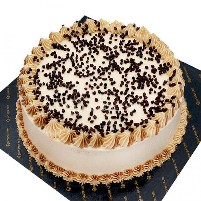
MATLAB 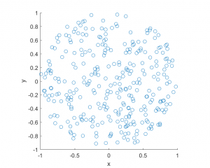
R 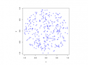
Python
Further reading
The third edition of the classic book Stochastic Geometry and its Applications by Chiu, Stoyan, Kendall and Mecke details on page 54 how to uniformly place points on a disk, which they call the radial way. The same simulation section appears in the previous edition by Stoyan, Kendall and Mecke (Chiu didn’t appear as an author until the current edition), though these books in general have little material on simulation methods. There is the book Spatial Point Patterns: Methodology and Applications with R written by spatial statistics experts Baddeley, Rubak and Turner, which covers the spatial statistics (and point process simulation) R-package spatstat.