I wrote this code a little while ago, and I thought now would be a good time to present it, as I have covered the topic of Markov chain Monte Carlo (MCMC) methods, particularly the central workhorse the Metropolis(-Rosenbluth-Rosenbluth-Teller-Teller)-Hastings algorithm. For more details on these methods, I have written about these methods in a couple posts, starting with this one and ending with this particularly relevant one.
Update: I re-wrote this code in C, located here, where I used my own code for generating Gaussian (or normal) variables, to keep the code entirely self-contained, but in practice you should never do that.
What the code does
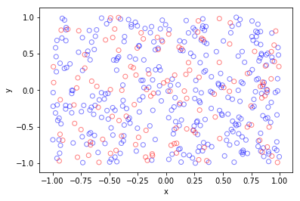
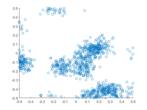
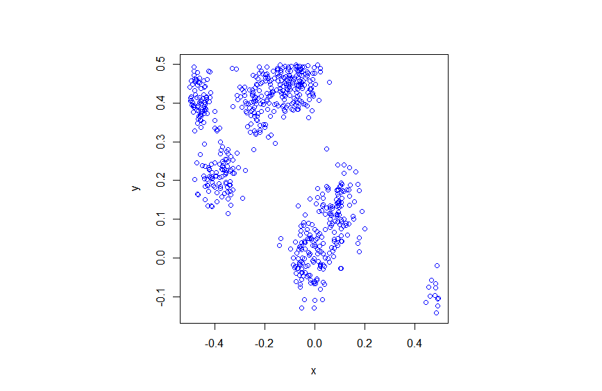
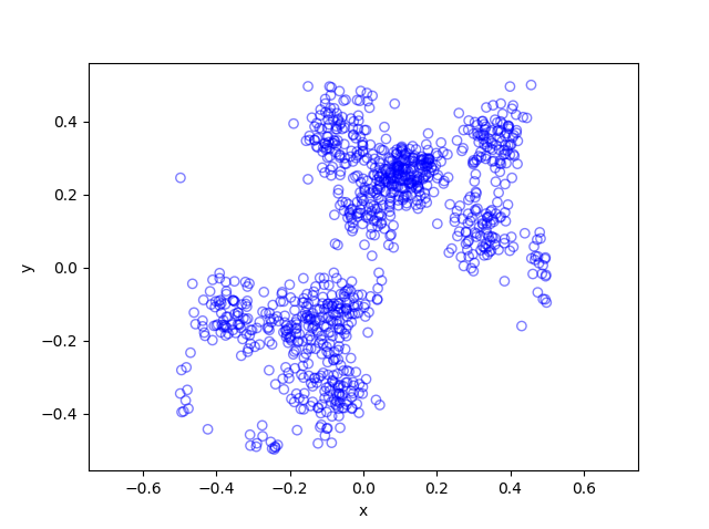
The code basically does the same thing in four different (scientific) programming languages, namely Python, Julia, C, and MATLAB. It performs a Metropolis-Hastings algorithm, simulating random variables (or more correctly, generating random variates) for two respective probabilities densities in one dimension and two dimensions.
Two examples
The one-dimensional case is particularly simple, as the code only simulates an exponential variable. But for this random variable in practice, you would never ever do with any MCMC method, because simply simulate exponential random variables directly. I discussed in a previous post how this direct approach is used to simulate Poisson variables.
The two-dimensional case is slightly more complicated than the the classic joint Gaussian (or normal) probability density, which you would use other methods to simulate. But the idea can be extended to \(n\) dimensions, which is often the case when dealing with the probability distributions and their corresponding integrals that arise in Bayesian statistics.
Implementation considerations
Variance of the walk
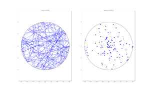
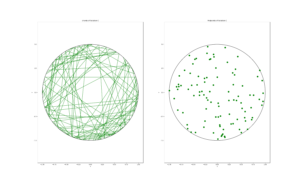
To create the random walk, the code uses normal (or Gaussian) random variables, where the mean is simply the current position of the random walk. This is a standard approach due to the convenient properties of normal distribution.
There’s also the standard deviation \(\sigma>0\) of the normal variables. In machine learning circles, this is what they call a hyperparameter. The random Metropolis-Hastings algorithm will, in theory, work regardless of the value, but some values result in faster results than others. This issue is covered briefly in this question on Stats Exchange. And it raises an important question when using MCMC methods in general.
Convergence tests
How many simulations steps are enough to ensure that the random variables being simulated behave closely enough to the desired random variables? In other words, how long does it take for the algorithm to target distribution?
The simulation time elapsed before the algorithm has reached a certain level of sufficient called the burn-in period. Due to its vital importance, it is a central topic in the development and implementation of MCMC methods.
There are tests for assessing the degree of convergence during the simulation run such as the Gelman-Rubin test. This particular test involves taking simple empirical means and variances over the last \(m\) samples, across all simulation runs, and between simulation runs. Then a ratio is calculated of variances is calculated, which should be close to one if the algorithm is sufficiently converged. I haven’t implemented any such tests here, but it’s something that one should do in practice.
Perhaps I’ll cover that topic in a future post.
Testing the results
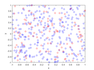
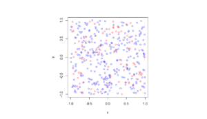
To test the results, you can empirical calculate the first two moments (that is, the mean and variance) of the simulated random variables. That acts as a very good sanity check.
But if you need more convincing, you can perform a histogram on the results, which effectively a way to empirically estimate the probability density of the simulated random variables. Fortunately, all four programming languages have built in histogram (counting) functions for one and two dimensions.
I already covered this topic in a previous posts on checking Poisson point process simulations.
Code
I’ll only include the code for Python and Julia, and refefr the reader to the rest of the code found here.
Python
I used the Matplotlib library to plot the probability density and its estimate.
For the histogram section, I used the histogram and histogram2d functions respectively to estimate the distribution of the number of points and the intensity function. I used the pdf option.
import numpy as np;  # NumPy package for arrays, random number generation, etc
import matplotlib.pyplot as plt  # for plotting
from matplotlib import cm  # for heatmap plotting
from mpl_toolkits import mplot3d  # for 3-D plots
from scipy import integrate  # for integrating

plt.close("all");  # close all previous plots

# Simulation window parameters
xMin = -1;
xMax = 1;
yMin = -1;
yMax = 1;

numbSim = 10 ** 4;  # number of random variables simulated
numbSteps = 200;  # number of steps for the Markov process
numbBins = 50;  # number of bins for histogram
sigma = 2;  # standard deviation for normal random steps

# probability density parameters
s = .5;  # scale parameter for distribution to be simulated

def fun_lambda(x, y):
    return np.exp(-(x ** 4 + x*y + y ** 2) / s ** 2);

# normalization constant
consNorm = integrate.dblquad(fun_lambda, xMin, xMax, lambda x: yMin, lambda y: yMax)[0];
#un-normalized joint density of variables to be simulated
def fun_p(x, y):
    return (fun_lambda(x, y) ) * (x >= xMin) * (y >= yMin) * (x <= xMax) * (y <= yMax);

xRand = np.random.uniform(xMin, xMax, numbSim);  # random initial values
yRand = np.random.uniform(yMin, yMax, numbSim);  # random initial values

pdfCurrent = fun_p(xRand, yRand);  # current transition (probability) densities

for jj in range(numbSteps):
    zxRand = xRand + sigma * np.random.normal(0, 1, numbSim);  # take a (normally distributed) random step
    zyRand = yRand + sigma * np.random.normal(0, 1, numbSim);  # take a (normally distributed) random step
    # Conditional random step needs to be symmetric in x and y
    # For example: Z|x ~ N(x,1) (or Y=x+N(0,1)) with probability density
    # p(z|x)=e(-(z-x)^2/2)/sqrt(2*pi)
    pdfProposal = fun_p(zxRand, zyRand);  # proposed probability

    # acceptance rejection step
    booleAccept = np.random.uniform(0, 1, numbSim) < pdfProposal / pdfCurrent;
    # update state of random walk/Markov chain
    xRand[booleAccept] = zxRand[booleAccept];
    yRand[booleAccept] = zyRand[booleAccept];
    # update transition (probability) densities
    pdfCurrent[booleAccept] = pdfProposal[booleAccept];

# for histogram, need to reshape as vectors
xRand = np.reshape(xRand, numbSim);
yRand = np.reshape(yRand, numbSim);

p_Estimate, xxEdges, yyEdges = np.histogram2d(xRand, yRand, bins=numbSteps, density=True);
xValues = (xxEdges[1:] + xxEdges[0:xxEdges.size - 1]) / 2;  # mid-points of bins
yValues = (yyEdges[1:] + yyEdges[0:yyEdges.size - 1]) / 2;  # mid-points of bins
X, Y = np.meshgrid(xValues, yValues);  # create x/y matrices for plotting

# analytic solution of (normalized) joint probability density
p_Exact = fun_p(X, Y) / consNorm;

# Plotting
# Plot empirical estimate
fig1 = plt.figure();
ax = plt.axes(projection="3d");
#plt.rc("text", usetex=True);
#plt.rc("font", family="serif");
surf = ax.plot_surface(X, Y, p_Estimate, cmap=plt.cm.plasma);
plt.xlabel("x");
plt.ylabel("y");
plt.title("p(x,y) Estimate");

# Plot exact expression
fig2 = plt.figure();
#plt.rc("text", usetex=True);
#plt.rc("font", family="serif")
ax = plt.axes(projection="3d");
surf = ax.plot_surface(X, Y, p_Exact, cmap=plt.cm.plasma);
plt.xlabel("x");
plt.ylabel("y");
plt.title("p(x,y) Exact Expression");
Julia
using Distributions #for random simulations
using PyPlot #for plotting
using StatsBase #for histograms etc
using Random
using LinearAlgebra
using HCubature #for numerical integration
#using LaTeXStrings #for LateX in labels/titles etc
PyPlot.close("all");  # close all PyPlot figures

#set random seed for reproducibility
#Random.seed!(1234)

# Simulation window parameters
xMin = -1;
xMax = 1;
yMin = -1;
yMax = 1;

numbSim = 10 ^ 5;  # number of random variables simulated
numbSteps = 25;  # number of steps for the Markov process
numbBins = 50;  # number of bins for histogram
sigma = 2;  # standard deviation for normal random steps

# probability density parameters
s = .5;  # scale parameter for distribution to be simulated

function fun_lambda(x,y)
    return (exp.(-(x.^4+x.*y+y.^2)./s^2));
end

#normalization constant -- UNDER CONSTRUCTION
consNorm,errorCub=hcubature(x -> fun_lambda(x[1],x[2]), [xMin, yMin], [xMax, yMax]);
#un-normalized joint density of variables to be simulated
function fun_p(x,y)
    return((fun_lambda(x,y)).*(x.>=xMin).*(y.>=yMin).*(x.<=xMax).*(y.<=yMax));
end
xRand=(xMax-xMin).*rand(numbSim).+xMin; #random initial values
yRand=(yMax-yMin).*rand(numbSim).+yMin; #random initial values

pdfCurrent=fun_p(xRand,yRand); #current transition (probability) densities
for jj=1:numbSteps
    zxRand= xRand.+sigma.*rand(Normal(),numbSim);#take a (normally distributed) random step
    zyRand= yRand.+sigma.*rand(Normal(),numbSim);#take a (normally distributed) random step

    # Conditional random step needs to be symmetric in x and y
    # For example: Z|x ~ N(x,1) (or Y=x+N(0,1)) with probability density
    # p(z|x)=e(-(z-x)^2/2)/sqrt(2*pi)
    pdfProposal = fun_p(zxRand, zyRand);  # proposed probability

    # acceptance rejection step
    booleAccept=rand(numbSim) .< pdfProposal./pdfCurrent;
    # update state of random walk/Markov chain
    xRand[booleAccept] = zxRand[booleAccept];
    yRand[booleAccept] = zyRand[booleAccept];
    # update transition (probability) densities
    pdfCurrent[booleAccept] = pdfProposal[booleAccept];
end

#histogram section: empirical probability density
histXY=fit(Histogram, (xRand,yRand),nbins=numbBins); #find histogram data
histXY=normalize(histXY,mode=:pdf); #normalize histogram
binEdges=histXY.edges; #retrieve bin edges
xValues=(binEdges[1][2:end]+binEdges[1][1:end-1])./2; #mid-points of bins
yValues=(binEdges[2][2:end]+binEdges[2][1:end-1])./2; #mid-points of bins
p_Estimate=(histXY.weights)
#create a meshgrid
X=[xValues[ii] for ii=1:length(xValues), jj=1:length(yValues)];
Y=[yValues[jj] for ii=1:length(xValues), jj=1:length(yValues)];

#analytic solution of (normalized) joint probability density
p_Exact = fun_p(X, Y)./consNorm;

# Plotting
# Plot empirical estimate
fig1 = PyPlot.figure();
PyPlot.rc("text", usetex=true);
PyPlot.rc("font", family="serif");
surf(X, Y, p_Estimate, cmap=PyPlot.cm.plasma);
PyPlot.xlabel("x");
PyPlot.ylabel("y");
PyPlot.title("p(x,y) Estimate");

# Plot exact expression
fig2 = PyPlot.figure();
PyPlot.rc("text", usetex=true);
PyPlot.rc("font", family="serif")
surf(X, Y, p_Exact, cmap=PyPlot.cm.plasma);
PyPlot.xlabel("x");
PyPlot.ylabel("y");
PyPlot.title("p(x,y) Exact Expression");