This work presents numerical results complementing mathematical work carried out by us. The work concerns (continuum) percolation results for a special network model based on Poisson-Voronoi tessellations.
The most relevant work are these two papers (the first being somewhat seminal):
Dousse, Franceschetti, Macris, Meester, Thiran, Percolation in the signal to interference ratio graph, 1996.
Le Gall, Błaszczyszyn, Cali, and En-Najjary, Continuum line-of-sight percolation on Poisson-Voronoi tessellations, 2021
Our work effectively seeks to combine these two papers. We obtain the equivalents results from the first paper by coupling its connectivity model with the connectivity model and network model (based on a Cox point process) presented in the second paper.
If you want a more detailed version, here’s the abstract:
To study the overall connectivity in device-to-device networks in cities, we incorporate a signal-to-interference-plus-noise connectivity model into a Poisson-Voronoi tessellation model representing the streets of a city. Relays are located at crossroads (or street intersections), whereas (user) devices are scattered along streets. Between any two adjacent relays, we assume data can be transmitted either directly between the relays or through users, given they share a common street. Our simulation results reveal that the network connectivity is ensured when the density of users (on the streets) exceeds a certain critical value. But then the network connectivity disappears when the user density exceeds a second critical value. The intuition is that for longer streets, where direct relay-to-relay communication is not possible, users are needed to transmit data between relays, but with too many users the interference becomes too strong, eventually reducing the overall network connectivity. This observation on the user density evokes previous results based on another wireless network model, where transmitter-receivers were scattered across the plane. This effect disappears when interference is removed from the model, giving a variation of the classic Gilbert model and recalling the lesson that neglecting interference in such network models can give overly optimistic results. For physically reasonable model parameters, we show that crowded streets (with more than six users on a typical street) lead to a sudden drop in connectivity. We also give numerical results outlining a relationship between the user density and the strength of any interference reduction techniques.
In future posts I’ll detail the above work as well as our more mathematical work on this type of percolation model.
Bowden, Keeler, Krzesinski, Taylor, Modeling and analysis of block arrival times in the Bitcoin blockchain, 2020.
This paper was based mostly on a previously uploaded preprint:
Bowden, Keeler, Krzesinski, Taylor, Block arrivals in the Bitcoin blockchain, 2018.
I briefly described this work in a previous post. We examined the arrivals of blocks in the Bitcoin blockchain by using both empirical (statistical) methods and mathematical (stochastic) models.
The paper builds off some previous work by us that uses a (relatively) new model in machine learning:
Błaszczyszyn and Keeler, Determinantal thinning of point processes with network learning applications.
https://arxiv.org/abs/1810.08672
The new machine learning model is based on a special type of point process called a determinantal point process. It was originally called a Fermion point process. These are useful point processes as the exhibit certain closure properties under certain operations such independent thinning.
Determinantal point processes are random objects and, when they are properly trained or fitted, can serve as generative artificial intelligence (or Gen AI) models. In fact, you can interpret these point processes as a special Gibbsian point processes, which have at their core a Hamiltonian function. A Hamiltonian is generalized type of energy function, which is also the basis for other generative (or stochastic) models such as Boltzmann machines.
In two previous posts, here and here, I discussed the importance of the quantity called the signal-to-interference ratio, which is usually abbreviated as SIR, for studying communication in wireless networks. In everyday terms, for a listener to hear a certain speaker in a room full of people speaking, the ratio of the speaker’s volume to the sum of the volumes of everyone else heard by the listener. The SIR is the communication bottleneck for any receiver and transmitter pair in a wireless network.
But the strengths (or power values) of the signals are of course also important. In this post I will detail how we can model them using a a simple network model with a single observer.
Propagation model
For a transmitter located at \(X_i\in \mathbb{R}^2\), researchers usually attempt to represent the received power of the signal \(P_i\) with a propagation model. Assuming the power is received at \(x\in \mathbb{R}^2\), this mathematical model consists of a random and a deterministic component taking the general form
$$
P_i(x)=F_i\,\ell(|X_i-x|) ,
$$
where \(\ell(r)\) is a non-negative function in \(r>0\) and \(F_i\) is a non-negative random variable.
The function \(\ell(r)\) is called the pathloss function, and common choices include \(\ell(r)=(\kappa r)^{-\beta}\) and \(\ell(r)=\kappa e^{-\beta r}\), where \(\beta>0\) and \(\kappa>0\) are model constants.
The random variables \(F_i\) represent signal phenomena such as multi-path fading and shadowing (also called shadow fading), caused by the signal interacting with the physical environment such as buildings. It is often called fading or shadowing variables.
We assume the transmitters locations \(X_1,\dots,X_n\) are on the plane \(\mathbb{R}^2\). Researchers typically assume they form a random point process or, more precisely, the realization of a random point process.
From two dimensions to one dimension
For studying wireless networks, a popular technique is to consider a wireless network from the perspective of a single observer or user. Researchers then consider the incoming or received signals from the entire network at the location of this observer or user. They do this by considering the inverses of the signal strengths, namely
Mathematically, this random function is simply a mapping from the two-dimensional plane \(\mathbb{R}^2\) to the one-dimensional non-negative real line \(\mathbb{R}_0^+=[0,\infty)\).
If the transmitters are located according to a non-random point pattern or a random point process, this random mapping generates a random point process on the non-negative real line. The resulting one-dimensional point process of the values \(L_1,L_2,\dots, \) has been called (independently) propagation (loss) process or path loss (with fading) process. More recently, my co-authors and I decided to call it a projection process, but of course the precise name doesn’t mattter
Intensity measure of signal strengths
Assuming a continuous monotonic path loss function \(\ell\) and the fading variables \(F_1, F_2\dots\) are iid, if the transmitters form a stationary random point process with intensity \(\lambda\), then the inverse signal strengths \(L_1,L_2,\dots \) form a random point process on the non-negative real line with the intensity measure \(M\).
where \(\ell^{-1}\) is the generalized inverse of the function \(\ell\). This expression can be generalized for a non-stationary point process with general intensity measure \(\Lambda\).
The inverses \(1/L_1,1/L_2,\dots \), which are the signal strengths, forprocess with intensity measure
Poisson transmitters gives Poisson signal strengths
Assuming a continuous monotonic path loss function \(\ell\) and the fading variables \(F_1, F_2\dots\) are iid, if the transmitters form a Poisson point process with intensity \(\lambda\), then the inverse signal strengths \(L_1,L_2,\dots \) form a Poisson point process on the non-negative real line with the intensity measure \(M\).
If \(L_1,L_2,\dots \) form a homogeneous Poisson point process, then the inverses \(1/L_1,1/L_2,\dots \) will also form a Poisson point process with intensity measure \(\bar{M}(s) =\lambda \pi \mathbb{E}( [\ell( F/s)^{-1} ]^2). \)
Propagation invariance
For \(\ell(r)=(\kappa r)^{-\beta}\) , the expression for the intensity measure \(M\) reduces to
$$
M(t) = \lambda \pi t^{-2/\beta} \mathbb{E}( F^{-2/\beta})/\kappa^2.
$$
What’s striking here is that information of the fading variable \(F\) is captured simply by one moment \(\mathbb{E}( F^{-2/\beta}) \). This means that two different distributions will give the same results as long as this moment is matching. My co-authors and I have been called this observation propagation invariance.
Some history
To study just the (inverse) signal strengths as a point process on the non-negative real line was a very useful insight. It was made independently in these two papers:
2008, Haenggi, A geometric interpretation of fading in wireless networks: Theory and applications;
2010, Błaszczyszyn, Karray, and Klepper, Impact of the geometry, path-loss exponent and random shadowing on the mean interference factor in wireless cellular networks.
My co-authors and I presented a general expression for the intensity measure \(M\) in the paper:
2018, Keeler, Ross and Xia, When do wireless network signals appear Poisson?.
This paper is also contains examples of various network models.
With Bartek Błaszczyszyn, Sayan Mukherjee, and Martin Haenggi, I co-wrote a short monograph on SINR models called Stochastic Geometry Analysis of Cellular Networks, which is written at a slightly more advanced level. The book puts an emphasis on studying the point process formed from inverse signal strengths, we call the projection process.
In the previous post I discussed the signal-to-interference-plus ratio or SIR in wireless networks. If noise is included, then then signal-to-interference-plus-noise ratio or just SINR. But I will just write about SIR, as most results that hold for SIR, will also hold for SINR without any great mathematical difficulty.
The SIR is an important quantity due to reasons coming from information theory. If you’re unfamiliar with it, I suggest reading the previous post.
In this post, I will describe a very popular mathematical model of the SIR, which I like to call the standard model. (This is not a term used in the literature as I have borrowed it from physics.)
Definition of SIR
To define the SIR, we consider a wireless network of \(n\) transmitters with positions located at \(X_1,\dots,X_n\) in some region of space. At some location \(x\), we write \(P_i(x)\) to denote the power value of a signal received at \(x\) from transmitter \(X_i\). Then at location \(x\), the SIR with respect to transmitter \(X_i\) is
$$
\text{SIR}(x,X_i) := \frac{P_i(x)}{\sum\limits_{j\neq i} P_j(x)} .
$$
Researchers usually attempt to represent the received power of the signal \(P_i(x)\) with a propagation model. This mathematical model consists of a random and a deterministic component given by
$$
P_i(x)=F_i\ell(|X_i-x|) ,
$$
where \(\ell(r)\) is a non-negative function in \(r\geq 0\) and \(F_i\) is a non-negative random variable. The function \(\ell(r)\) is often called the path loss function. The random variables represent random fading or shadowing.
Standard model
Based on the three model components of fading, path loss, and transmitter locations, there are many combinations possible. That said, researchers generally (I would guess, say, 90 percent or more) use a single combination, which I call the standard model.
The three standard model assumptions are:
Singular power law path loss \(\ell(r)=(\kappa r)^{-\beta}\).
Why these three? Well, in short, because they work very well together. Incredibly, it’s sometimes possible to get relatively a simple mathematical expression for, say, the coverage probability \(\mathbb{P}[\text{SIR}(x,X_i)>\tau ]\), where \(\tau>0\).
I’ll now detail the reasons more specifically.
Path loss
The \(\ell(r)=(\kappa r)^{-\beta}\) is very simple, despite having a singularity at \(r=0\). This allows simple algebraic manipulation of equations.
Some, such as myself, are initially skeptical of this function as it gives an infinitely strong signal at the transmitter due to the singularity in the function \(\ell(r)=(\kappa r)^{-\beta}\). More specifically, the path loss of the signal from transmitter \(X_i\) approaches infinity as \(x\) approaches \(X_i\) .
But apparently, overall, the singularity does not have a significant impact on most mathematical results, at least qualitatively. That said, one still observe consequences of this somewhat physically unrealistic model assumption. And I strongly doubt enough care is taken by researchers to observe and note this.
Fading and shadowing variables
Interestingly, the original reason why exponential variables were used is because it allowed the SIR problem to be reformulated into a problem of a Laplace transform of a random variable, which for a random variable \(Y\) is defined as
The reason for this connection is that the tail distribution of an exponential variable \(F\) with mean \(\mu\) is simply \(\mathbb{P}(F>t)= e^{-t/\mu}\). In short, with the exponential assumption, various conditioning arguments eventually lead to Laplace transforms of random variables.
Transmitters locations
No prizes for guessing that researcher overwhelmingly use a (homogeneous) Poisson point process for the transmitter (or receiver) locations. When developing mathematical models with point processes, if you can’t get any results with the Poisson point process, then abandon all hope.
It’s the easier to work with this point process due to its independence property, which leads to another useful property. For Poisson point process, the Palm distribution is known, which is the distribution of a point process conditioned on a point (or collection of points) existing in a specific location of the underlying space on which the point process is defined. In general, the Palm distribution is not known for many point processes.
Random propagation effects can lead to Poisson
A lesser known reason why researchers would use the Poisson point process is that, from the perspective of a single observer in the network, it can be used to capture the randomness in the signal strengths. Poisson approximation results in probability imply that randomly perturbing the signal strengths can make signals appear more Poisson, by which I mean the signal strengths behave stochastically or statistically as though they were created by a Poisson network of transmitters.
The end result is that a non-Poisson network can appear more Poisson, even if the transmitters do not resemble (the realization of) a Poisson point process. The source of randomness that makes a non-Poisson network appear more Poisson is the random propagation effects of fading, shadowing, randomly varying antenna gains, and so on, or some combination of these.
2009, Haenggi, Andrews, Baccelli, Dousse, Franceschetti, Stochastic Geometry and Random Graphs for the Analysis and Design of Wireless Networks.
This paper by my co-authors and I has some details on standard model and why a general network model behaving Poisson in terms of the signal strengths:
2018, Keeler, Ross and Xia, When do wireless network signals appear Poisson?.
Finally, I co-wrote with Bartek Błaszczyszyn, Sayan Mukherjee, and Martin Haenggi a short monograph on SINR models called Stochastic Geometry Analysis of Cellular Networks, which is written at a slightly more advanced level. This book has a section on why signal strengths appear Poisson.
Basic information theory says that for a signal to successfully communicate across any communication link, the signal strength must be stronger than that of the background noise, leading to the fundamental quantity known as signal-to-noise ratio. Information theory holds in very general (or, in mathematical speak, abstract) settings. The communication could be, for example, a phone call on an old wired landline, two people talking in a bar, or a hand-written letter, for which the respective signals in these examples are the electrical current, speaker’s voice, and the writing. (Respective examples of noise could be, for example, thermal noise in the wires, loud music, or coffee stains on the letter.)
In wireless networks, it’s possible for a receiver to simultaneously detect signals from multiple transmitters, but the receiver typically only wants to receive one signal. The other unwanted or interfering signals form a type of noise, which is usually called interference, and the other (interfering) transmitters are called interferers. Consequently, researchers working on wireless networks study the signal-to-interference ratio, which is usually abbreviated as SIR. Another name for the SIR is carrier-to-interference ratio.
If we also include background noise, which is coming not from the interferers, then the quantity becomes the signal-to-interference-plus-noise ratio or just SINR. But I will just write about SIR, though jumping from SIR to SINR is usually not difficult mathematically.
The concept of SIR makes successful communication more difficult to model and predict, as it just doesn’t depend on the distance of the communication link. Putting the concept in everyday terms, for a listener to hear a certain speaker in a room full of people all speaking to the listener, it is not simply the distance to the speaker, but rather the ratio of the speaker’s volume to the sum of the volumes of everyone else heard by the listener. The SIR is the communication bottleneck for any receiver and transmitter pair in a wireless network.
In wireless network research, much work has been done to examine and understand communication success in terms of interference and SIR, which has led to a popular mathematical model that incorporates how signals propagate and the locations of transmitters and receivers.
Definition
To define the SIR, we consider a wireless network of transmitters with positions located at \(X_1,\dots,X_n\) in some region of space. At some location \(x\), we write \(P_i(x)\) to denote the power value of a signal received at \(x\) from transmitter \(X_i\). Then at location \(x\), the SIR with respect to transmitter \(X_i\) is
$$
\text{SIR}(x,X_i) :=\frac{P_i(x)}{\sum\limits_{j\neq i} P_j(x)} =\frac{P_i(x)}{\sum\limits_{j=1}^{n} P_j(x)-P_i(x)} .
$$
The numerator is the signal and the denominator is the interference. This ratio tells us that increasing the number of transmitters \(n\) decreases the original SIR values. But then, in exchange, there is a greater number of transmitters for the receiver to connect to, some of which may have larger \(P_i(x)\) values and, subsequently, SIR values. This delicate trade-off makes it challenging and interesting to mathematically analyze and design networks that deliver high SIR values.
Researchers usually assume that the SIR is random. A quantity of interest is the tail distribution of the SIR, namely
where \(\tau>0\) is some parameter, sometimes called the SIR threshold. For a given value of \(\tau\), the probability \(\mathbb{P}[\text{SIR}(x,X_i)>\tau]\) is sometimes called the coverage probability, which is simply the probability that a signal coming from \(X_i\) can be received successfully at location \(x\).
Mathematical models
Propagation
Researchers usually attempt to represent the received power of the signal \(P_i(x)\) with a propagation model. This mathematical model consists of a random and a deterministic component taking the general form
$$
P_i(x)=F_i\ell(|X_i-x|) ,
$$
where \(F_i\) is a non-negative random variable and \(\ell(r)\) is a non-negative function in \(r \geq 0\).
Path loss
The function \(\ell(r)\) is called the path loss function, and common choices include \(\ell(r)=(\kappa r)^{-\beta}\) and \(\ell(r)=\kappa e^{-\beta r}\), where \(\beta>0\) and \(\kappa>0\) are model constants, which need to be fitted to (or estimated with) real world data.
Researchers generally assume that the so-called path loss function \(\ell(r)\) is decreasing in \(r\), but actual path loss (that is, the change in signal strength over a path travelled) typically increases with distance \(r\). Researchers originally assumed path loss functions to be increasing, not decreasing, giving the alternative (but equivalent) propagation model
$$
P_i(x)= F_i/\ell(|X_i-x|).
$$
But nowadays researchers assume that the function \(\ell(r)\) is decreasing in \(r\). (Although, based on personal experience, there is still some disagreement on the convention.)
Fading and shadowing
With the random variable \(F_i\), researchers seek to represent signal phenomena such as multi-path fading and shadowing (also called shadow fading), caused by the signal interacting with the physical environment such as buildings. These variables are often called fading or shadowing variables, depending on what physical phenomena they are representing.
Typical distributions for fading variables include the exponential and gamma distributions, while the log-normal distribution is usually used for shadowing. The entire collection of fading or shadowing variables is nearly always assumed to be independent and identically distributed (iid), but very occasionally random fields are used to include a degree of statistical dependence between variables.
Transmitters locations
In general, we assume the transmitters locations \(X_1,\dots,X_n\) are on the plane \(\mathbb{R}^2\). To model interference, researchers initially proposed non-random models, but they were considered inaccurate and intractable. Now researchers typically use random point processes or, more precisely, the realizations of random point processes for the transmitter locations.
Not surprisingly, the first natural choice is the Poisson point process. Other point processes have been used such as Matérn and Thomas cluster point processes, and Matérn hard-core point processes, as well as determinantal point processes, which I’ll discuss in another post.
Some history
Early random models of wireless networks go back to the 60s and 70s, but these were based simply on geometry: meaning a transmitter could communicate successfully to a receiver if they were closer than some fixed distance. Edgar Gilbert created the field of continuum percolation with this significant paper:
1961, Gilbert, Random plane networks.
Interest in random geometrical models of wireless networks continued into the 70s and 80s. But there was no SIR in these models.
Motivated by understanding SIR, researchers in the late 1990s and early 2000s started tackling SIR problems by using a random model based on techniques from stochastic geometry and point processes. Early papers include:
1997, Baccelli, Klein, Lebourges ,and Zuyev, Stochastic geometry and architecture of communication networks;
2003, Baccelli and Błaszczyszyn , On a coverage process ranging from the Boolean model to the Poisson Voronoi tessellation, with applications to wireless communications;
2006, Baccelli, Mühlethaler, and Błaszczyszyn, An Aloha protocol for multihop mobile wireless networks.
But they didn’t know that some of their results had already been discovered independently by researchers working on wireless networks in the early 1990s. These papers include:
1994, Pupolin and Zorzi, Outage probability in multiple access packet radio networks in the presence of fading;
1990, Sousa and Silvester, Optimum transmission ranges in a direct-sequence spread-spectrum multihop packet radio network.
The early work focused more on small-scale networks like wireless ad hoc networks. Then the focus shifted dramatically to mobile or cellular phone networks with the publication of the paper:
2011, Andrews, Baccelli, Ganti, A tractable approach to coverage and rate in cellular networks.
It’s can be said with confidence that this paper inspired much of the interest in using point processes to develop models of wireless networks. The work generally considers the SINR in the downlink channel for which the incoming signals originate from the phone base stations.
Finally, Bartek Błaszczyszyn, Sayan Mukherjee, Martin Haenggi, and I wrote a short book on SINR models called Stochastic Geometry Analysis of Cellular Networks, which is written at a slightly more advanced level. The book puts an emphasis on studying the point process formed from inverse signal strengths, which we call the projection process.
Cholera outbreaks due to public water pumps. Suburbs serviced by hospitals. Formation of crystals. Coverage regions of phone towers. We can model or approximate all these phenomena and many, many more with a geometric structure called, among other names, a Voronoi tessellation.
To form a Voronoi tessellation, consider a collection of points scattered on some space, like the plane, where it’s easier to picture things, especially when using a Euclidean metric. Now for each point in the collection, consider the surrounding region that is closer to that point than any other point in the collection. Each region forms a cell corresponding to the point. The union of all the sets covers the underlying space. That union of sets is the Voronoi tessellation.
The evolution of Voronoi cells, which start off as disks until they collide with each other. Source: Wikipedia.
Mathematicians have extensively studied Voronoi tessellations, particularly those based on Poisson point processes, forming a core subject in the field of stochastic geometry.
It’s also called a Dirichlet tessellation
The main other name for the Voronoi tessellation is the Dirichlet tessellation. Historically, Dirichlet beats Voronoi, but it seems wherever I look, the name Voronoi usually wins out, suggesting an example of Stigler’s law of eponymy. A notable exception is the R library spatstat that does actually call it a Dirichlet tessellation. Wikipedia calls it a Voronoi diagram. I’ve read that Descartes studied the object even earlier than Dirichlet, but Voronoi studied it in much more depth. At any rate, I will call it a Voronoi tessellation.
Everyday Voronoi tessellations
Voronoi tessellations are just not interesting mathematical objects, as they arise in everyday situations. This piece from Scientific American website explains:
Everyone uses Voronoi tessellations, even without realizing it. Individuals seeking the nearest café, urban planners determining service area for hospitals, and regional planners outlining school districts all consider Voronoi tessellations. Each café, school, or hospital is a site from which a Voronoi tessellation is generated. The cells represent ideal service areas for individual businesses, schools, or hospitals to minimize clientele transit time. Coffee drinkers, patients, or students inside a service area (that is, a cell) should live closer to their own café, hospital, or school (that is, their own cell’s site) than any other. Voronoi tessellations are ubiquitous, yet often invisible.
Delaunay triangulation
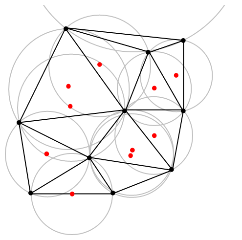
A closely related object is the Delaunay triangulation. For a given collection of points on some underlying mathematical space, a Delaunay triangulation is formed by connecting the points and creating triangles with the condition that for each point, no other point exists in the circumcircle of the corresponding triangle. (A circumcircle is a circle that passes through all three vertices of a triangle.)
An example of Delaunay triangulation with the original points in black and centrers (in red) of the corresponding circumcircles (in grey) of the Delaunay triangles. Source: Wikipedia.
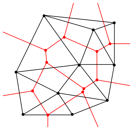
The vertices of the the Delaunay triangular and Voronoi tessellation both form graphs, which turn out to be the dual graphs of each other.
A Delaunay triangulation (in black) and the corresponding Voronoi tessellation (in red) whose vertices are the centres of the circumcircles of the Delaunay triangles. Source: Wikipedia.
Software: Qhull
Due to its applications, it’s not surprising that there exist algorithms that quickly create or estimate Voronoi tessellations. I don’t want to implement one of these algorithms from scratch, as they have already been implemented in various scientific programming languages. Many of the languages, such as MATLAB, R, and Python (SciPy) use the code from Qhull. (Note the Qhull website calls the tessellation a Voronoi diagram.)
(The Julia programming language, which I examined in a previous post, has a Voronoi package that does not use Qhull.)
Qhull finds the Voronoi tessellation by first finding the Delaunay triangulation. If the underlying space is bounded, then all the Voronoi cells are also bounded. But on an unbounded space, it is possible to have unbounded cells, meaning their areas (or volumes) are infinite. In such cases, the algorithms sometime place virtual points at infinity, but I don’t want to focus on such details. I will assume Qhull does a good job.
Code
As always, the code from all my posts is online. For this post, the MATLAB and Python code is here and here, respectively, which generates Voronoi tesselations.
MATLAB
It is fairly straightforward to create Voronoi tessellations in MATLAB. You can just use the function voronoi, which is only for two-dimensional tessellations. (Note: the MATLAB website says the behaviour of the function voronoi has changed, so that may cause problems when using different versions of MATLAB.) The function requires two inputs as vectors, say, x and y, corresponding to the Cartesian (or \(x\) and \(y\)) coordinates of the points. If you just run the voronoi command, it will create and plot a Voronoi tessellation (or Voronoi diagram, as MATLAB calls it). But the MATLAB website also describes how to plot the tessellation manually.
For \(d\) -dimensional tessellations, there is the function voronoin, which requires a single input. The single output consists of combining \(d\) column vectors for the Cartesian coordinates. For example, given the column vectors x, y and z, then the input is [x, y, z].
If you give the functions voronoi or voronoin output arguments, then the tessellation is not plotted and instead two data structures, say, v and c are created for describing the vertices of the tessellation. I generally use voronoi for plotting, but I use voronoin (and not voronoi) for generating vertex data, so I will focus on the outputs of voronoin.
For voronoin, the first (output) data structure v is simply an two-dimensional array array that contain the Cartesian coordinates of every vertex in the Voronoi tessellation. The second (output) data structure c is a cell array describing the vertices of each Voronoi cell (it has to be a cell array, as opposed to a regular array, as the cells have varying number of vertices). Each entry of the cell array contains a one-dimensional array with array indices corresponding to the \(x\) and \(y\) coordinates.
The code checks which Voronoi cells are unbounded by seeing if they have vertices at infinity, which corresponds to a \(1\) in the index arrays (stored in the structure array c).
One criticism of the MATLAB functions is that they don’t return all the information of the Voronoi tessellation. More specifically, the functions don’t return the boundaries between the unbounded cells, though voronoi internally calculates and uses these boundaries to generate Voronoi plots. This is covered in this review on different Voronoi packages. Conversely, the Python package returns more information such as that of the edges or ridges of the Voronoi cells.
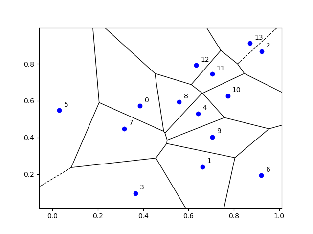
Python
To create the Voronoi tessellation, use the SciPy (Spatial) function Voronoi. This function does \(d\)-dimensional tessellations. For the two-dimensional setting, you need to input the \(x\) and \(y\) coordinates as a single array of dimensions \(2 \times n\), where \(n\) is the number of points in the collection. In my code, I start off with two one-dimensional arrays for the Cartesian coordinates, but then I combined them into a single array by using the function numpy.stack with the function argument axis =1.
I would argue that the Voronoi function in SciPy is not as intuitive to use as the MATLAB version. One thing I found a bit tricky, at first, is that the cells and the points have a different sets of numbering (that is, they are indexed differently). (And I am not the only one that was caught by this.) You must use the attribute called point_region to access a cell number (or index) from a point number (or index). In my code the attribute is accessed and then called it indexP2C, which is an integer array with cell indices. Of course, there could be a reason for this, and I am just failing to understand it.
Apart from the above criticism, the function Voronoi worked well. As I mentioned before, this package returns more Voronoi information than the MATLAB equivalents.
To plot the Voronoi tessellation, use the SciPy function voronoi_plot_2d, which allows for various plotting options, but it does require Matplotlib. The input is the data object created by the function Voronoi.
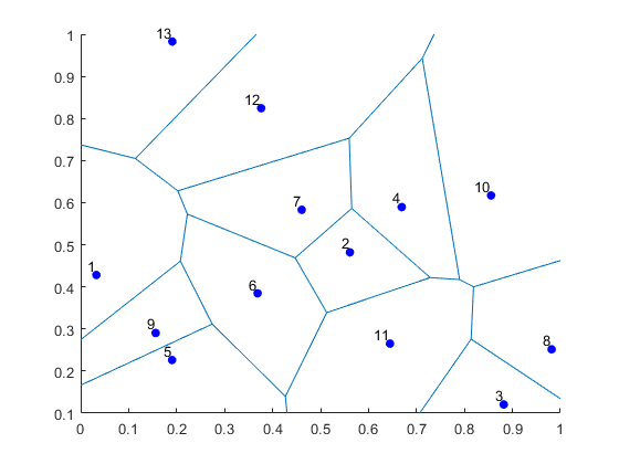
Results
I’ve plotted the results for a single realization of a Poisson point process. I’ve also plotted the indices of the points. Recall that the indexing in Python and MATLAB start respectively at zero and one.
MATLAB
Python
Voronoi animations
I took the animation of evolving Voronoi cells, which appears in the introduction, from Wikipedia. The creator generated it in MATLAB and also posted the code online. The code is long, and I wouldn’t even dare to try to reproduce it, but I am glad someone else wrote it.
Such animations exist also for other metrics. For example, the Manhattan metric (or taxi cab or city block metric) gives the animation below, where the growing disks have been replaced with squares.
A Voronoi tessellation under the Manhattan metric. The evolving cells start off as squares until they collide with each other. Source: Wikipedia.
This Wikipedia user page has animations under other metrics on Euclidean space.
This post also features animations of Voronoi tessellations when the points move.
Further reading
There is a lot of literature on Voronoi or Dirichlet tessellations, particularly when the seeds of the cells form a Poisson point process. The references in the articles on Wikipedia and MathWorld are good starting points.
Here is a good post on Voronoi tesselations. Here is a non-mathematical article published in the Irish Times.
Google Scholar has requested me to make available a freely available copy of this published comment my former PhD supervisor and I wrote a few years ago:
Keeler and Taylor, Some remarks regarding “On the Laplace Transform of the Aggregate Discounted Claims with Markovian arrivals”
OK, Google Scholar, here’s the manuscript that we submitted, which is basically the same as the published version.
The comment and the original paper cover an insurance model (for aggregate claims) that uses a Markov arrival process. Such stochastic processes use matrix theory. But there was a small error in the original paper, where commutativity had been assumed, which is clearly not the case in general for matrices. Despite this error, the incorrect solution gave surprisingly accurate answers, so we investigated why that was.
Nothing groundbreaking here by us. We were just curious.
The paper uses a (relatively) new model framework in machine learning. This framework is based on a special type of point process called a determinantal point process, which is also called a fermion point process. (This particle model draw inspiration from the form of the wave function in quantum mechanics.) Kulesza and Taskar introduced and developed the framework for using determinantal point processes for machine learning models.
The paper covers a type of generative machine learning (or Gen AI) model, due to its using randomness to create network outcomes. In fact, you can interpret these point processes as a special Gibbsian point processes, which have at their core a Hamiltonian function. A Hamiltonian is generalized type of energy function, which is also the basis for other generative (or stochastic) models such as Boltzmann machines.
The training method for determinantal point processes is based on the maximum likelihood approach, which gives a convex optimization problem, allowing you to tackle it with your favourite gradient method, such as the BFGS or Adam method.
It turns out that point processes are amenable for looking at the signal-to-inference-plus-noise ratio (SINR) — see this post for details. More specifically, we found these point processes give tractable SINR-based expressions when you use (what I call) the standard (SINR) model, which I covered in a previous post.
Code
The MATLAB code for the producing the results in the paper can be found here:
My collaborators and I later extended this line of work in a separate paper, where we looked at the problem of designing a smart(er) medium access control (MAC) scheduling algorithm:
Błaszczyszyn, Brochard, and Keeler, Coverage probability in wireless networks with determinantal scheduling.


