Stochastic geometry Archives

Voronoi tessellations in architecture

A colleague just sent me this photo of a colourful building on the Gold Coast. The building is the new Home of the Arts (HOTA) Gallery, as detailed here. It is covered in a Voronoi tessellation. I described this very useful geometrical object in a previous post.

The New HOTA Gallery with a Voronoi tessellation on the outside.

A casual Google reveals that other buildings have Voronoi-inspired architecture. For example, The Fry building at the University of Bristol in Britain, which fittingly houses the mathematics department.

The Fry Building at the University of Bristol (Source)

The building for the Alibaba headquarters in China also evokes Voronoi imagery. But those Voronoi constructions do no feature the colours of the HOTA Gallery, which is reminiscent of diagrams produced by scientific plotting packages.

(Of course I don’t mind the odd Voronoi tesselation. For example, a couple of months ago I set for my website image a Voronoi tesselation, created by the Franco-German artist Plaisance Puisatier. And the cover of a book I co-wrote has a diagram based on the signal-to-interference ratio, which can be considered as a generalization of a Voronoi tessellation.)

Mathematical buildings

Another building that employs an interesting geometrical object is RMIT’s Storey Hall, located in Melbourne. It features Penrose tiling, which is an example of a non-periodic tiling. Loosely speaking, that means if you tile an infinite plane with a given a set of tiles, then no translation of the plane will yield the same pattern again. The Penrose tiling is also inside the building, as you can see on this website.

On topic of non-periodic tiling, the buildings at Federation Square in Melbourne are covered by pinwheel tiling, as shown on this mathematics website, which is also non-periodic. According to Wikipedia, Charles Radin proposed this tiling based on a construction by the late and famous John Conway who died earlier this year, being yet another victim of the pandemic.

Mathematical architects

While writing this post, I noticed that both the HOTA Gallery and Storey Hall were designed by ARM Architecture. Some of their other buildings have a geometrical aspect. Clearly they have a mathematical inclination.

Point processes

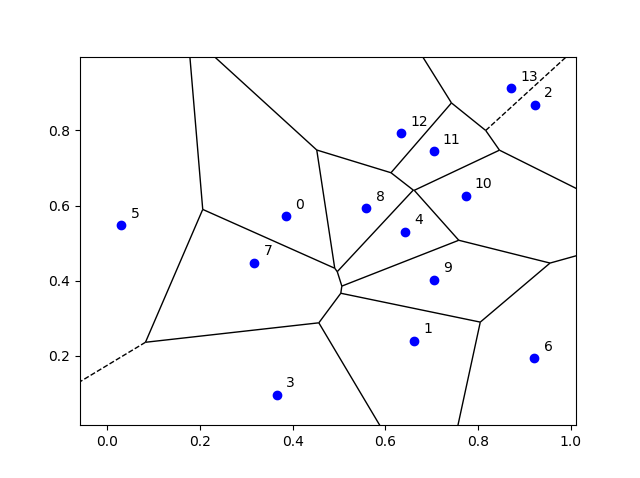
A non-random collection of points located on some space is called a point pattern in spatial statistics. Informally, you can interpret a point process as a collection of random points scattered over some underlying mathematical space, meaning each outcome or realization of a point process forms a point pattern. Using such intuition gets you pretty far. But if we want to be mathematically formal, we need to use precise mathematical objects.

Historically, there’s a couple main interpretations of a point process, which is also called a random point field. But now a standard mathematical approach is used.

In this post I will cover the main definitions, terminology and some of the notation used in the theory and application of point processes. (I refer to the next post for more on the point process notation.) I won’t delve too much into the precise details, giving just an outline with references at the end.

Underlying mathematical space

We consider a point process defined on some underlying mathematical space $\mathbb{S}$, which is sometimes called the carrier space or state space. We further assume that the space is measurable by having a Borel $\sigma$-algebra $\mathcal{S}$.

In practice, the underlying space is usually the real line $\mathbb{R}$, the plane $\mathbb{R}^2$, or some other familiar mathematical space like a square lattice. More generally, a point process can be defined on any metric space, allowing for the notion of distance. Mathematicians study point processes in even more general settings by defining them on, for example, a locally compact second countable Hausdorff space. But such generality is typically not needed for most people and their applications.

Modern probability approach

In modern probability theory, if we want to define a random mathematical object, we start with a random experiment in the context of a probability space or triple $(\Omega,\mathcal{A},\mathbb{P})$, where:

$\Omega$ is a sample space, which is the set of all possible outcomes;
$\mathcal{A}$ is a $\sigma$-algebra or $\sigma$-field, which is a family of events (subsets of $\Omega$);
$\mathbb{P}$ is a probability measure, which assigns probability to each event in $\mathcal{A}$.

To gain some intuition, David Williams says to imagine that Tyche, Goddess of Chance, chooses a sample point $\omega\in\Omega$ at random according to the law $\mathbb{P}$ such that an event $A\in \mathcal{A}$ has a probability given by $\mathbb{P}(A)$, where we understand probability with our own intuition. To bring things back to Earth, we can also choose a sample point $\omega\in\Omega$ by using some physical experiment, as long as it is truly random, such that the probability of $A\in \mathcal{A}$ happening is given by $\mathbb{P}(A)$.

Now we can define random objects by using a certain measurable function or mapping that maps to a suitable space of objects. For example, a real-valued random variable is a measurable function from $\Omega$ to the real line; a random matrix is a measurable function from $\Omega$ to some space of matrices; and, as John Kingman quips in his classic book Poisson Processes, a random elephant is just a measurable function from $\Omega$ to some suitable space of elephants.

But what space should we use for a point process? To answer that, we need to interpret a point process as a suitable mathematical object.

Interpretation

There are different ways to interpret a point process, which is often denoted by a single letter, for example, $N$ or $\Phi$. (The convention of using the Greek letter $\Phi$ comes from German mathematicians, but some prefer not to use $\Phi$, as it’s often used for the normal cumulative distribution function.) If the point process is defined on a space like the real like, where the points can be ordered, then additional interpretations exist, but mathematicians assume the order of the points does not matter, limiting the possible interpretations.

Random closed set

In mathematics a collection of distinct things is formalized by a mathematical object called a set. We say that a set contains elements or members, and a set never contains more than one of the same element. Sets are fundamental objects with set concepts and notation being found everywhere in mathematics.

We now define a common type of point process, which we can formalize with the concept of a set.

A point process is simple if the probability of all points of the point process being distinct is one.

In other words, for a simple point process, there is zero probability of two or more of its points being found in the same location of the underlying state space $\mathbb{S}$, which brings us to our first interpretation.

A simple point process can be interpreted as a random closed set.

More specifically, we can interpret a simple point process as a (measurable) mapping from a sample space $\Omega$ to the space of closed sets $\mathbb{F}$, meaning that each realization of a simple point process is a closed set $\phi\in \mathbb{F}$.

Point process theory has adopted the notation from set theory. For example, if we want to say some point, which we denote by $x$, of the underlying space $\mathbb{S}$ belongs to or is a member of a simple point process $\Phi$, then we can simply write $x\in \Phi$. We can also write a point process as $\{x\}_i$ to highlight its interpretation as a random closed set of points.

The theory of random sets, which is a field of study in its own right, can be applied to simple point processes owing to this interpretation. But for non-simple point processes, we need another point process interpretation.

Random measures

Modern integration theory is based on measure theory, which revolves around the concept of a set function known as a measure. In addition to a couple of other properties, when you apply this function to a set, it gives a number, such as a integer or real number. For example, a counting measure gives you the number elements in a set, which could be a subspace $B$, such as a region of the plane $B \subset \mathbb{R}^2$. (The letter $B$ is often used for sets in measure and probability theory as it’s typically assumed that the sets are Borel sets, which form a very large family of well-behaved sets in terms of measurability.) The concept of a counting measure gives us an interpretation of a point process, which has now become the standard one.

A point process can be interpreted a random counting measure.

More specifically, we define a point process as a mapping from a sample space $\Omega$ to the space of counting measures $\mathbb{M}$, meaning that each realization of a point process is a counting measure $\phi\in \mathbb{M}$. Some mathematicians even say a point process is just another name for a random counting measure. The techniques of random measure theory provide alternative (and arguably main) approach to study point processes.

This standard interpretation of a point process means that point process theory borrows heavily notation from measure theory and calculus. For example, in measure theory we can write a (non-random) counting measure as $\#$, so $\#(B)=n$ is how we write that the set $B$ contains $n$ points. We can then write the the number of points of a point process $\Phi$ located in some (Borel) set $B$ as $N(B) =\#( B \cap \Phi)$, where $N(B)$ is a random variable. In this expression, the point process is denoted by $\Phi$, while$N(B)$ is the number of points of $\Phi$ in $B$, meaning $N$ is a random counting measure .

Important concepts

In the theory point processes, like any other field of mathematics, there are various important concepts for understanding and proving various results. Without going in the details, these include shot noise, Campbell’s theorem, Laplace functional, Palm calculus, void probability, and factorial moment measures. In future posts, I’ll detail some of these concepts.

Signal-to-interference ratio in wireless networks

The fundamentals of information theory say that to successfully communicate across any potential communication link the signal strength of the communication must be stronger than that of the back ground noise, which leads to the fundamental quantity known as signal-to-noise ratio. Information theory holds in very general (or, in mathematical speak, abstract) settings. The communication could be, for example, a phone call on an old wired landline, two people talking in a bar, or a hand-written letter, for which the respective signals in these examples are the electrical current, speaker’s voice, and the writing. (Respective examples of noise could be, for example, thermal noise in the wires, loud music, or coffee stains on the letter.)

In wireless networks, it’s possible for a receiver to simultaneously detect signals from multiple transmitters, but the receiver typically only wants to receive one signal. The other unwanted or interfering signals form a type of noise, which is usually called interference, and the other (interfering) transmitters are called interferers. Consequently, researchers working on wireless networks study the signal-to-interference ratio, which is usually abbreviated as SIR. Another name for the SIR is carrier-to-interference ratio.

If we also include background noise, which is coming not from the interferers, then the quantity becomes the signal-to-interference-plus-noise ratio or just SINR. But I will just write about SIR, though jumping from SIR to SINR is usually not difficult mathematically.

The concept of SIR makes successful communication more difficult to model and predict, as it just doesn’t depend on the distance of the communication link. Putting the concept in everyday terms, for a listener to hear a certain speaker in a room full of people all speaking to the listener, it is not simply the distance to the speaker, but rather the ratio of the speaker’s volume to the sum of the volumes of everyone else heard by the listener. The SIR is the communication bottleneck for any receiver and transmitter pair in a wireless network.

In wireless network research, much work has been done to examine and understand communication success in terms of interference and SIR, which has led to a popular mathematical model that incorporates how signals propagate and the locations of transmitters and receivers.

Definition

To define the SIR, we consider a wireless network of transmitters with positions located at $X_1,\dots,X_n$ in some region of space. At some location $x$, we write $P_i(x)$ to denote the power value of a signal received at $x$ from transmitter $X_i$. Then at location $x$, the SIR with respect to transmitter $X_i$ is
$$
\text{SIR}(x,X_i) :=\frac{P_i(x)}{\sum\limits_{j\neq i} P_j(x)} =\frac{P_i(x)}{\sum\limits_{j=1}^{n} P_j(x)-P_i(x)} .
$$

The numerator is the signal and the denominator is the interference. This ratio tells us that increasing the number of transmitters $n$ decreases the original SIR values. But then, in exchange, there is a greater number of transmitters for the receiver to connect to, some of which may have larger $P_i(x)$ values and, subsequently, SIR values. This delicate trade-off makes it challenging and interesting to mathematically analyze and design networks that deliver high SIR values.

Researchers usually assume that the SIR is random. A quantity of interest is the tail distribution of the SIR, namely

$$
\mathbb{P}[\text{SIR}(x,X_i)>\tau ] := \frac{P_i(x)}{\sum\limits_{j\neq i} P_j(x)} \,,
$$

where $\tau>0$ is some parameter, sometimes called the SIR threshold. For a given value of $\tau$, the probability $\mathbb{P}[\text{SIR}(x,X_i)>\tau]$ is sometimes called the coverage probability, which is simply the probability that a signal coming from $X_i$ can be received successfully at location $x$.

Mathematical models

Propagation

Researchers usually attempt to represent the received power of the signal $P_i(x)$ with a propagation model. This mathematical model consists of a random and a deterministic component taking the general form
$$
P_i(x)=F_i\ell(|X_i-x|) ,
$$
where $F_i$ is a non-negative random variable and $\ell(r)$ is a non-negative function in $r \geq 0$.

Path loss

The function $\ell(r)$ is called the path loss function, and common choices include $\ell(r)=(\kappa r)^{-\beta}$ and $\ell(r)=\kappa e^{-\beta r}$, where $\beta>0$ and $\kappa>0$ are model constants, which need to be fitted to (or estimated with) real world data.

Researchers generally assume that the so-called path loss function $\ell(r)$ is decreasing in $r$, but actual path loss (that is, the change in signal strength over a path travelled) typically increases with distance $r$. Researchers originally assumed path loss functions to be increasing, not decreasing, giving the alternative (but equivalent) propagation model
$$
P_i(x)= F_i/\ell(|X_i-x|).
$$

But nowadays researchers assume that the function $\ell(r)$ is decreasing in $r$. (Although, based on personal experience, there is still some disagreement on the convention.)

Fading and shadowing

With the random variable $F_i$, researchers seek to represent signal phenomena such as multi-path fading and shadowing (also called shadow fading), caused by the signal interacting with the physical environment such as buildings. These variables are often called fading or shadowing variables, depending on what physical phenomena they are representing.

Typical distributions for fading variables include the exponential and gamma distributions, while the log-normal distribution is usually used for shadowing. The entire collection of fading or shadowing variables is nearly always assumed to be independent and identically distributed (iid), but very occasionally random fields are used to include a degree of statistical dependence between variables.

Transmitters locations

In general, we assume the transmitters locations $X_1,\dots,X_n$ are on the plane $\mathbb{R}^2$. To model interference, researchers initially proposed non-random models, but they were considered inaccurate and intractable. Now researchers typically use random point processes or, more precisely, the realizations of random point processes for the transmitter locations.

Not surprisingly, the first natural choice is the Poisson point process. Other point processes have been used such as Matérn and Thomas cluster point processes, and Matérn hard-core point processes, as well as determinantal point processes, which I’ll discuss in another post.

Some history

Early random models of wireless networks go back to the 60s and 70s, but these were based simply on geometry: meaning a transmitter could communicate successfully to a receiver if they were closer than some fixed distance. Edgar Gilbert created the field of continuum percolation with this significant paper:

1961, Gilbert, Random plane networks.

Interest in random geometrical models of wireless networks continued into the 70s and 80s. But there was no SIR in these models.

Motivated by understanding SIR, researchers in the late 1990s and early 2000s started tackling SIR problems by using a random model based on techniques from stochastic geometry and point processes. Early papers include:

1997, Baccelli, Klein, Lebourges ,and Zuyev, Stochastic geometry and architecture of communication networks;
2003, Baccelli and Błaszczyszyn , On a coverage process ranging from the Boolean model to the Poisson Voronoi tessellation, with applications to wireless communications;
2006, Baccelli, Mühlethaler, and Błaszczyszyn, An Aloha protocol for multihop mobile wireless networks.

But they didn’t know that some of their results had already been discovered independently by researchers working on wireless networks in the early 1990s. These papers include:

1994, Pupolin and Zorzi, Outage probability in multiple access packet radio networks in the presence of fading;
1990, Sousa and Silvester, Optimum transmission ranges in a direct-sequence spread-spectrum multihop packet radio network.

The early work focused more on small-scale networks like wireless ad hoc networks. Then the focus shifted dramatically to mobile or cellular phone networks with the publication of the paper:

2011, Andrews, Baccelli, Ganti, A tractable approach to coverage and rate in cellular networks.

It’s can be said with confidence that this paper inspired much of the interest in using point processes to develop models of wireless networks. The work generally considers the SINR in the downlink channel for which the incoming signals originate from the phone base stations.

Placing a random point uniformly in a Voronoi cell

In the previous post, I discussed how Voronoi or Dirichlet tesselations are useful and how they can be calculated or estimated with many scientific programming languages by using standard libraries usually based on Qhull. The cells of such a tessellation divide the underlying space. Now I want to randomly place a single point in a uniform manner in each bounded Voronoi cell.

But why?

Well, this task arises occasionally, particularly when developing mathematical models of wireless networks, such as mobile or cellular phone networks. A former colleague of mine had to do this, which inspired me to write some MATLAB code a couple of years ago. And I’ve seen the question posed a couple of times on the web . So I thought: I can do that.

Overview

For this problem, I see two obvious methods.

Simple but crude

The simplest method is to cover each Voronoi cell with a rectangle or disk. Then randomly place a point uniformly on the rectangle or disk. If it doesn’t randomly land inside the rectangle or disk, then do it again until it does. Crude, slightly inefficient, but simple.

Elegant but slightly tricky

A more elegant way, which I will implement, is to partition (or divide) each Voronoi cell into triangles. Then randomly choose a triangle based on its area and, finally, uniformly position a point on that triangle.

Method

Partition cells into triangles

It is straightforward to divide a Voronoi cell into triangles. Each side of the cell corresponds to one side of a triangle (that is, two points). The third point of the triangle is the original point corresponding to the Voronoi cell.

Choose a triangle

Randomly choosing a triangle is also easy. For a given cell, number the triangles. Which random triangle is chosen is simply a discrete random variable whose probability mass function is formed from triangle areas normalized (or divided) by the total area of the Voronoi cell. In other words, the probability of randomly choosing triangle $i$ with area $A_i$ from $m$ triangles is simply

$P_i=\frac{A_i}{\sum_{j=1}^m A_j}.$

To calculate the area of the triangles, I use the shoelace formula , which for a triangle with corners labelled $\textbf{A}$, $\textbf{B}$ and $\textbf{C}$ gives

$A= \frac{1}{2} |(x_{\textbf{B}}-x_{\textbf{A}})(y_{\textbf{C}}-y_{\textbf{A}})-(x_{\textbf{C}}-x_{\textbf{A}})(y_{\textbf{B}}-y_{\textbf{A}})|.$

But you can also use Herron’s formula.

Then the random variable is sampled using the probabilities based on the triangle areas.

Place point on chosen triangle

Given a triangle, the final step is also easy, if you know how, which is often the case in mathematics. I have already covered this step in a previous post, but I’ll give some details here.

To position a single point uniformly in the triangle, generate two random uniform variables on the unit interval $(0,1)$, say $U$ and $V$. The random $X$ and $Y$ coordinates of the single point are given by the expressions:

$X=\sqrt{U} x_{\textbf{A}}+\sqrt{U}(1-V x_{\textbf{B}})+\sqrt{U}V x_{\textbf{C}}$

$Y=\sqrt{U} y_{\textbf{A}}+\sqrt{U}(1-V y_{\textbf{B}})+\sqrt{U}V y_{\textbf{C}}$

Results

The blue points are the points of the underlying point pattern that was used to generate the Voronoi tesselation. (These points have also been arbitrarily numbered.) The red points are the random points that have been uniformly placed in all the bounded Voronoi cells.

MATLAB

Python

Empirical validation

We can empirically validate that the points are being placed uniformly on the bounded Voronoi cells. For a given (that is, non-random) Voronoi cell, we can repeatedly place (or sample) a random point uniformly in the cell. Increasing the number of randomly placed points, the respective averages of the $x$ and $y$ coordinates of the points will converge to the centroids (or geometric centres) of the Voronoi cell, which can be calculated with simple formulas.

Code

The code for all my posts is located online here. For this post, the code in MATLAB and Python is here.

I have also written in MATLAB and Python the code as functions (in files funVoronoiUniform.m and funVoronoiUniform.py, respectively), so people can use it more easily. The function files are located here, where I have also included an implementation of the aforementioned empirical test involving centroids. You should be able to use those functions and for any two-dimensional point patterns.

Voronoi tessellations

Cholera outbreaks due to public water pumps. Suburbs serviced by hospitals. Formation of crystals. Coverage regions of phone towers. We can model or approximate all these phenomena and many, many more with a geometric structure called, among other names, a Voronoi tessellation.

The main other name for this object is the Dirichlet tessellation. Historically, Dirichlet beats Voronoi, but it seems wherever I look, the name Voronoi usually wins out, suggesting an example of Stigler’s law of eponymy. A notable exception is the R library spatstat that does actually call it a Dirichlet tessellation. Wikipedia calls it a Voronoi diagram. I’ve read that Descartes studied the object even earlier than Dirichlet, but Voronoi studied it in much more depth. At any rate, I will call it a Voronoi tessellation.

To form a Voronoi tessellation, consider a collection of points scattered on some space, like the plane, where it’s easier to picture things, especially when using a Euclidean metric. Now for each point in the collection, consider the surrounding region that is closer to that point than any other point in the collection. Each region forms a cell corresponding to the point. The union of all the sets covers the underlying space. That union of sets is the Voronoi tessellation.

The evolution of Voronoi cells, which start off as disks until they collide with each other. Source: Wikipedia.

Mathematicians have extensively studied Voronoi tessellations, particularly those based on Poisson point processes, forming a core subject in the field of stochastic geometry.

Everyday Voronoi tessellations

Voronoi tessellations are just not interesting mathematical objects, as they arise in everyday situations. This piece from Scientific American website explains:

Everyone uses Voronoi tessellations, even without realizing it. Individuals seeking the nearest café, urban planners determining service area for hospitals, and regional planners outlining school districts all consider Voronoi tessellations. Each café, school, or hospital is a site from which a Voronoi tessellation is generated. The cells represent ideal service areas for individual businesses, schools, or hospitals to minimize clientele transit time. Coffee drinkers, patients, or students inside a service area (that is, a cell) should live closer to their own café, hospital, or school (that is, their own cell’s site) than any other. Voronoi tessellations are ubiquitous, yet often invisible.

Delaunay triangulation

A closely related object is the Delaunay triangulation. For a given collection of points on some underlying mathematical space, a Delaunay triangulation is formed by connecting the points and creating triangles with the condition that for each point, no other point exists in the circumcircle of the corresponding triangle. (A circumcircle is a circle that passes through all three vertices of a triangle.)

The vertices of the the Delaunay triangular and Voronoi tessellation both form graphs, which turn out to be the dual graphs of each other.

A Delaunay triangulation (in black) and the corresponding Voronoi tessellation (in red) whose vertices are the centres of the circumcircles of the Delaunay triangles. Source: Wikipedia.

Software: Qhull

Due to its applications, it’s not surprising that there exist algorithms that quickly create or estimate Voronoi tessellations. I don’t want to implement one of these algorithms from scratch, as they have already been implemented in various scientific programming languages. Many of the languages, such as MATLAB, R, and Python (SciPy) use the code from Qhull. (Note the Qhull website calls the tessellation a Voronoi diagram.)

(The Julia programming language, which I examined in a previous post, has a Voronoi package that does not use Qhull.)

Qhull finds the Voronoi tessellation by first finding the Delaunay triangulation. If the underlying space is bounded, then all the Voronoi cells are also bounded. But on an unbounded space, it is possible to have unbounded cells, meaning their areas (or volumes) are infinite. In such cases, the algorithms sometime place virtual points at infinity, but I don’t want to focus on such details. I will assume Qhull does a good job.

Code

As always, the code from all my posts is online. For this post, the MATLAB and Python code is here and here, respectively, which generates Voronoi tesselations.

MATLAB

It is fairly straightforward to create Voronoi tessellations in MATLAB. You can just use the function voronoi, which is only for two-dimensional tessellations. (Note: the MATLAB website says the behaviour of the function voronoi has changed, so that may cause problems when using different versions of MATLAB.) The function requires two inputs as vectors, say, x and y, corresponding to the Cartesian (or $x$ and $y$) coordinates of the points. If you just run the voronoi command, it will create and plot a Voronoi tessellation (or Voronoi diagram, as MATLAB calls it). But the MATLAB website also describes how to plot the tessellation manually.

For $d$ -dimensional tessellations, there is the function voronoin, which requires a single input. The single output consists of combining $d$ column vectors for the Cartesian coordinates. For example, given the column vectors x, y and z, then the input is [x, y, z].

If you give the functions voronoi or voronoin output arguments, then the tessellation is not plotted and instead two data structures, say, v and c are created for describing the vertices of the tessellation. I generally use voronoi for plotting, but I use voronoin (and not voronoi) for generating vertex data, so I will focus on the outputs of voronoin.

For voronoin, the first (output) data structure v is simply an two-dimensional array array that contain the Cartesian coordinates of every vertex in the Voronoi tessellation. The second (output) data structure c is a cell array describing the vertices of each Voronoi cell (it has to be a cell array, as opposed to a regular array, as the cells have varying number of vertices). Each entry of the cell array contains a one-dimensional array with array indices corresponding to the $x$ and $y$ coordinates.

The code checks which Voronoi cells are unbounded by seeing if they have vertices at infinity, which corresponds to a $1$ in the index arrays (stored in the structure array c).

One criticism of the MATLAB functions is that they don’t return all the information of the Voronoi tessellation. More specifically, the functions don’t return the boundaries between the unbounded cells, though voronoi internally calculates and uses these boundaries to generate Voronoi plots. This is covered in this review on different Voronoi packages. Conversely, the Python package returns more information such as that of the edges or ridges of the Voronoi cells.

Python

To create the Voronoi tessellation, use the SciPy (Spatial) function Voronoi. This function does $d$-dimensional tessellations. For the two-dimensional setting, you need to input the $x$ and $y$ coordinates as a single array of dimensions $2 \times n$, where $n$ is the number of points in the collection. In my code, I start off with two one-dimensional arrays for the Cartesian coordinates, but then I combined them into a single array by using the function numpy.stack with the function argument axis =1.

I would argue that the Voronoi function in SciPy is not as intuitive to use as the MATLAB version. One thing I found a bit tricky, at first, is that the cells and the points have a different sets of numbering (that is, they are indexed differently). (And I am not the only one that was caught by this.) You must use the attribute called point_region to access a cell number (or index) from a point number (or index). In my code the attribute is accessed and then called it indexP2C, which is an integer array with cell indices. Of course, there could be a reason for this, and I am just failing to understand it.

Apart from the above criticism, the function Voronoi worked well. As I mentioned before, this package returns more Voronoi information than the MATLAB equivalents.

To plot the Voronoi tessellation, use the SciPy function voronoi_plot_2d, which allows for various plotting options, but it does require Matplotlib. The input is the data object created by the function Voronoi.

Results

I’ve plotted the results for a single realization of a Poisson point process. I’ve also plotted the indices of the points. Recall that the indexing in Python and MATLAB start respectively at zero and one.

MATLAB

Python

Voronoi animations

I took the animation of evolving Voronoi cells, which appears in the introduction, from Wikipedia. The creator generated it in MATLAB and also posted the code online. The code is long, and I wouldn’t even dare to try to reproduce it, but I am glad someone else wrote it.

Such animations exist also for other metrics. For example, the Manhattan metric (or taxi cab or city block metric) gives the animation below, where the growing disks have been replaced with squares.

A Voronoi tessellation under the Manhattan metric. The evolving cells start off as squares until they collide with each other. Source: Wikipedia.

This Wikipedia user page has animations under other metrics on Euclidean space.

This post also features animations of Voronoi tessellations when the points move.

Mathematical buildings

Mathematical architects

Underlying mathematical space

Modern probability approach

Interpretation

Random closed set

Random measures

Important concepts

Further reading

Definition

Mathematical models

Propagation

Path loss

Fading and shadowing

Transmitters locations

Some history

Further reading

Overview

Simple but crude

Elegant but slightly tricky

Method

Partition cells into triangles

Choose a triangle

Place point on chosen triangle

Results

MATLAB

Python

Empirical validation

Code

Further reading

Everyday Voronoi tessellations

Delaunay triangulation

Software: Qhull

Code

MATLAB

Python

Results

MATLAB

Python

Voronoi animations

Further reading