There’s an old saying, which I just made up. If you really want to understand something, code it up in C.1Taking it to the next level, I recall an undergraduate subject on programming Motorola chips using assembly. But I wouldn’t recommend any of that.
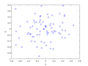
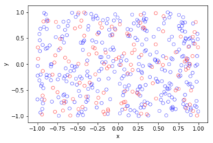
I wrote some C code that basically does what my code in this previous post does without the pretty pictures. The code performs a Metropolis-Hastings algorithm, simulating random variables (or, more correctly, generating random variates) for a joint probability density describing two random variables.
In previous posts, I have covered the topic of Markov chain Monte Carlo (MCMC) methods, particularly the central workhorse, the Metropolis(-Rosenbluth-Rosenbluth-Teller-Teller)-Hastings algorithm. These methods are frequently used in Bayesian statistics, high-dimensional integration, and optimization. For more details on how they work, I have written a couple posts, starting with this one and ending with this one, where I detail the mechanics of MCMC methods.
Let’s call this code MCMC C code2 Wise man once wrote: C:/DOS C:/DOS/RUN RUN/DOS/RUN.
Code considerations
The C programming language was not written for playing with random numbers. The standard uniform random number generator in C, simply called rand, is not good for research level random simulations. But it does the job for illustration purposes.
In lieu of this generator, the Mersenne Twister is a popular algorithm for producing such numbers, which is widely recommended and used. There are implementations of this algorithm in the CUDA and MKL libraries for Nvidia GPUs and Intel CPUs; see this CUDA page and this MKL page for details. Check out this PDF file for further details on the CUDA version.
In addition to that, my C code needs to simulate normal (or Gaussian) random variables. For that I wrote my own simple code using the Box-Muller transform, which I covered in a previous post, so the code would be self-contained and less opaque. But in reality, you should always use functions from a pre-written library for generating variates according to a normal or whichever distribution.
Finally, C was never intended as a scientific language, despite its wide use as one. (Historically, that was Fortran’s job, which is still the workhorse for many serious number-crunching institutes, hence why there’s Fortran -ready version of CUDA.) So when handling sets of numbers, such as vectors and matrices, one has to use pointers and malloc more often that not, which can be a tricky. This is the case here, though the use of pointers in this code is relatively simple.
Where are the pretty pictures?
Unfortunately, when number crunching in C, you don’t immediately have access to plotting libraries that are available in scientific programming languages such as Python and Julia.
But you can simply create .csv (or text) files, and then plot them using whichever library you prefer. And if you have gnuplot installed, you can perform simple one-dimensional histograms using one-line commands such as:
gnuplot -e “plot ‘MCMCData_1D.csv’ using 1 bins=20;” -persist
In the above command, the file MCMCData_1D.csv has the random variates (the simulated random variables) stored in a single column.
Code
I only present code for the more complicated two-dimensional case. The code can be found here.
Note that there’s an option in the code of MCMC_1D.c to plot the results using gnuplot, if it’s installed on your machine. I didn’t include code for plotting the results of the 2-D case as gnuplot doesn’t do a 2-D histogram.
Warning: The code uses the standard pseudo-random number generator in C, which is known for being bad. I only used built-in the C generator to keep my code self-contained. For that reason, I also wrote my code for generating Gaussian (or normal) random variables, by using the Box-Muller transform, but in reality one would never do that for research or industry purposes.
/***********************************************************************
 * Runs a simple Metropolis-Hastings (ie MCMC) algorithm to simulate two
 * jointly distributed random variables with probability density
 * p(x,y)=exp(-(x^4+x*y+y^2)/s^2)/consNorm, where s>0 and consNorm is a
 * normalization constant. The probability density function is defined in
 * the function pdf_single.
 *
 * NOTE: In practice, the value of the normalization constant is not needed, as it cancels out in the algorithm.
 *
 * NOTE: This code will *create* a local file (see variable strFilename) to store results. It will *overwrite* that file if it already exists.
 *
 * WARNING: This code uses the default C random number generator, which is known for failing various tests of randomness.
 * Strongly recommended to use another generator for purposes beyond simple illustration.
 *
 * Author: H. Paul Keeler, 2024.
 * Website: hpaulkeeler.com
 * Repository: github.com/hpaulkeeler/posts
 *
 ***********************************************************/

#include <stdio.h>
#include <stdlib.h>
#include <time.h>
#include <math.h>
#include <stdbool.h>
#include <string.h>

const long double pi = 3.14159265358979323846; // constant pi for generating polar coordinates

// helper function declarations; see below for definitions
static double *unirand(double *randValues, unsigned numbRand);                           // generate  uniform random variables on (0,1)
static double *normrand(double *randValues, unsigned numbRand, double mu, double sigma); // generate normal random variables
static double pdf_single(double x, double y, double s);                      // define probability density to be simulated
static double mean_var(double *set_sample, unsigned numbSim, double *varX);              // calculate meana and variance

int main(int argc, char *argv[])
{

    if (argc > 1)
    {
        fprintf(stderr, "This program takes no arguments...\n");
        exit(1);
    }
    else
    {

        char strFilename[] = "MCMCData_2D.csv"; // filename for storing simulated random variates

        // intializes (pseudo)-random number generator
        time_t timeCPU; // use CPU time for seed
        srand((unsigned)time(&timeCPU));
        // srand(42); //to reproduce results

        bool booleWriteData = true; // write data to file
        bool booleStats = true;     // perform simple mean/std stats

        // parameters
        unsigned numbSim = 1e4;   // number of random variables simulated
        unsigned numbSteps = 200; // number of steps for the Markov process
        double sigma = 2;         // standard deviation for normal random steps

        // probability density parameters
        double s = .5; // scale parameter for distribution to be simulated

        // Metropolis-Hastings variables
        // proposal for a new position in the random walk
        double zxRandProposal;
        double zyRandProposal;
        double pdfProposal; // density for proposed position
        double pdfCurrent;  // density of current position
        double ratioAccept; // ratio of densities (ie acceptance probability)
        double uRand;       // uniform variable for Bernoulli trial (ie a coin flip)
        // random step (normally distributed)
        double *p_numbNormX = (double *)malloc(1 * sizeof(double));
        double *p_numbNormY = (double *)malloc(1 * sizeof(double));
//positions of the random walk (ie the simualted random variables after numbSteps)
        double *p_xRand = (double *)malloc(numbSim * sizeof(double));
        double *p_yRand = (double *)malloc(numbSim * sizeof(double));

        (void)unirand(p_xRand, numbSim); // random initial values
        (void)unirand(p_yRand, numbSim); // random initial values

        unsigned i, j; // loop varibales
        for (i = 0; i < numbSim; i++)
        {
            // loop through each random walk instance (or random variable to be simulated)

            pdfCurrent = pdf_single(*(p_xRand + i), *(p_yRand + i), s); // current probability density

            for (j = 0; j < numbSteps; j++)
            {
                // loop through each step of the random walk
                (void)normrand(p_numbNormX, 1, 0, sigma);
                (void)normrand(p_numbNormY, 1, 0, sigma);
                // take a(normally distributed) random step in x and y
                zxRandProposal = (*(p_xRand + i)) + (*p_numbNormX);
                zyRandProposal = (*(p_yRand + i)) + (*p_numbNormY);

                pdfProposal = pdf_single(zxRandProposal, zyRandProposal, s); // proposed probability density

                // acceptance rejection step
                (void)unirand(&uRand, 1);
                ratioAccept = pdfProposal / pdfCurrent;
                if (uRand < ratioAccept)
                {
                    // update state of random walk / Markov chain
                    *(p_xRand + i) = zxRandProposal;
                    *(p_yRand + i) = zyRandProposal;
                    pdfCurrent = pdfProposal;
                }
            }
        }

        free(p_numbNormX);
        free(p_numbNormY);

        if (booleStats)
        {

            // initialize statistics variables (for testing results)
            char strVariable[] = "XY";
            double *p_AllRand[] = {p_xRand, p_yRand};
            double meanTemp = 0;
            double varTemp = 0;
            double stdTemp = 0;
            char strTemp='X';
            for (i = 0; i < 2; i++)
            {
                meanTemp = mean_var(p_AllRand[i], numbSim, &varTemp);
                stdTemp = sqrt(varTemp);
                strTemp=strVariable[i];
                printf("The average of the %c random variables is %lf.\n", strTemp, meanTemp);
                printf("The standard deviation of the %c random  variables is %lf.\n", strTemp, stdTemp);
            }
        }

        if (booleWriteData)
        {
            // print to file
            FILE *outputFile;
            outputFile = fopen(strFilename, "w");
            for (i = 0; i < numbSim; i++)
            {
                fprintf(outputFile, "%lf,%lf\n", *(p_xRand + i), *(p_yRand + i)); // output to file
            }
            fclose(outputFile);
            printf("Data printed to file.\n");
        }
        free(p_xRand);
        free(p_yRand);

        return (0);
    }
}

static double pdf_single(double x, double y, double s)
{
    // returns the probability density of a single point (x,y) inside a simulation window defined below
    double pdf_output;

    // non-zero density window parameters
    double xMin = -1;
    double xMax = 1;
    double yMin = -1;
    double yMax = 1;

    if ((x >= xMin) && (x <= xMax) && (y >= yMin) && (y <= yMax))
    {
        pdf_output = exp(-((pow(x, 4) + x * y + pow(y, 2)) / (s * s)));
    }
    else
    {
        pdf_output = 0;
    }
    return pdf_output;
}

static double *normrand(double *randValues, unsigned numbRand, double mu, double sigma)
{
    // simulate pairs of iid normal variables using Box-Muller transform
    // https://en.wikipedia.org/wiki/Box%E2%80%93Muller_transform

    double U1, U2, thetaTemp, rhoTemp, Z1, Z2;
    int i = 0;
    while (i < numbRand)
    {
        // simulate variables in polar coordinates (theta, rho)
        (void)unirand(&U1, 1);
        thetaTemp = 2 * pi * U1; // create uniform theta values
        (void)unirand(&U2, 1);
        rhoTemp = sqrt(-2 * log(U2)); // create Rayleigh rho values

        // change to Cartesian coordinates
        Z1 = rhoTemp * cos(thetaTemp);
        Z1 = sigma * Z1 + mu;
        randValues[i] = Z1; // assign first of random variable pair
        i++;
        if (i < numbRand)
        {
            // if more variables are needed, generate second value of random pair
            Z2 = rhoTemp * sin(thetaTemp);
            Z2 = sigma * Z2 + mu;
            randValues[i] = Z2; // assign second of random variable pair
            i++;
        }
        else
        {
            break;
        }
    }
    return randValues;
}

static double *unirand(double *randValues, unsigned numbRand)
{ // simulate numbRand uniform random variables on the unit interval
  // storing them in randValues which must be allocated by the caller
  // with enough space for numbRand doubles

    for (int i = 0; i < numbRand; i++)
    {
        randValues[i] = (double)rand() / RAND_MAX;
    }
    return randValues;
}

static double mean_var(double *set_sample, unsigned numbSim, double *varX)
{
    // mean and variance of set_sample
    int i;
    // initialize statistics variables (for testing results)
    double meanX = 0;
    double meanXSquared = 0;
    double tempX;
    for (i = 0; i < numbSim; i++)
    {
        tempX = *(set_sample + i);
        meanX += tempX / ((double)numbSim);
        meanXSquared += tempX * tempX / ((double)numbSim);
    }

    *varX = meanXSquared - meanX * meanX;
    return meanX;
}
Further reading
Here’s some information on the rand function and random number generation:
- https://codeforces.com/blog/entry/61587
- https://c-faq.com/lib/randrange.html
- https://www.codeproject.com/KB/recipes/pitfalls_random_number.aspx
Acknowledg(e)ments
A hat tip to C and CUDA guru Alex Stivala who pointed out a couple of minor issues in my original C code.