In previous posts I have often stressed the importance of the Poisson point process as a mathematical model. But it can be unsuitable for certain mathematical models. We can generalize it by first considering a non-negative random measure, called a driving or directing measure. Then a Poisson point process, which is independent of the random driving measure, is generated by using the random measure as its intensity or mean measure. This doubly stochastic construction gives what is called a Cox point process.
In practice we don’t typically observe the driving measure. This means that it’s impossible to distinguish a Cox point process from a Poisson point process if there’s only one realization available. By conditioning on the random driving measure, we can use the properties of the Poisson point process to derive those of the resulting Cox point process.
By the way, Cox point processes are also known as doubly stochastic Poisson point processes. Guttorp and Thorarinsdottir argue that we should call them the Quenouille point processes, as Maurice Quenouille introduced an example of it before Sir David Cox. But I opt for the more common name.
In this post I’ll cover a couple examples of Cox point processes. But first I will need to give a more precise mathematical definition.
Definition
We consider a point process defined on some underlying mathematical space \(\mathbb{S}\), which is sometimes called the carrier space or state space. The underlying space is often the real line \(\mathbb{R}\), the plane \(\mathbb{R}^2\), or some other familiar mathematical space like a square lattice.
For the first definition, we use the concept of a random measure.
Let \(M\) be a non-negative random measure on \(\mathbb{S} \). Then a point process \(\Phi\) defined on some underlying space \(\mathbb{S}\) is a Cox point process driven by the intensity measure \(M\) if the conditional distribution of \(\Phi\) is a Poisson point process with intensity function \(M\).
We can give a slightly less general definition of a Cox point process by using a random intensity function.
Let \(Z=\{Z(x):x\in\mathbb{S} \}\) be a non-negative random field such that with probability one, \(x\rightarrow Z(x)\) is a locally integrable function. Then a point process \(\Phi\) defined on some underlying space \(\mathbb{S}\) is a Cox point process driven by \(Z\) if the conditional distribution of \(\Phi\) is a Poisson point process with intensity function \(Z\).
The random driving measure \(M\) is then simply the integral
$$
M(B)=\int_B Z(x)\, dx , \quad B\subseteq S.
$$
Over-dispersion
The random driving measures take different forms, giving different Cox point processes. But there is a general observation that can be made for all Cox point processes. For any region \(B \subseteq S\), it can be shown that the number of points \(\Phi (B)\) adheres to the inequality
$$
\mathbb{Var} [\Phi (B)] \geq \mathbb{E} [\Phi (B)],
$$
where \(\mathbb{Var} [\Phi (B)] \) is the variance of the random variable \(\Phi (B)\). As a comparison, for a Poisson point process \(\Phi’\), the variance of \(\Phi’ (B)\) is simply \(\mathbb{Var} [\Phi’ (B)] =\mathbb{E} [\Phi’ (B)]\). Due to its greater variance, the Cox point process is said to be over-dispersed compared to the Poisson point process.
Special cases
There is an virtually unlimited number of ways to define a random driving measure, where each one yields a different a Cox point process. But in general we are restricted by examining only tractable and interesting Cox point processes. I will give some common examples, but I stress that the Cox point process family is very large.
Mixed Poisson point process
For the random driving measure \(M\), an obvious example is the product form \(M= Y \mu \), where \(Y\) is some independent non-negative random variable and \(\mu\) is the Lebesgue measure on \(\mathbb{S}\). This driving measure gives the mixed Poisson point process. The random variable \(Y\) is the only source of randomness.
Log-Gaussian Cox point process
Instead of a random variable, we can use a non-negative random field to define a random driving measure. We then have the product \(M= Y \mu \), where \(Y\) is now some independent non-negative random field. (A random field is a collection of random variables indexed by some set, which in this case is the underlying space \(\mathbb{S}\).)
Arguably the most tractable and used random field is the Gaussian random field. This random field, like Gaussian or normal random variables, takes both negative and positive values. But if we define the random field such that its logarithm is a Gaussian field \(Z\), then we obtain the non-negative random driving measure \(M=\mu e^Z \), giving the log-Gaussian Cox point process.
This point process has found applications in spatial statistics.
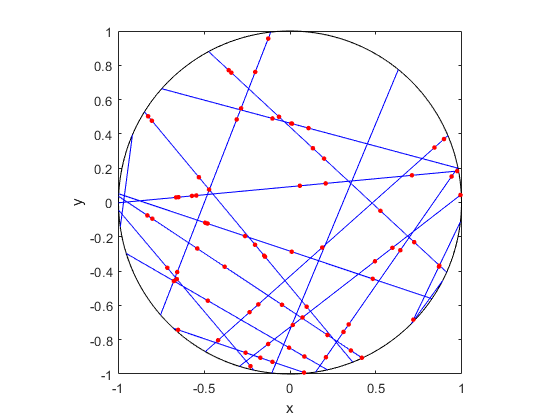
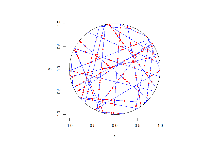
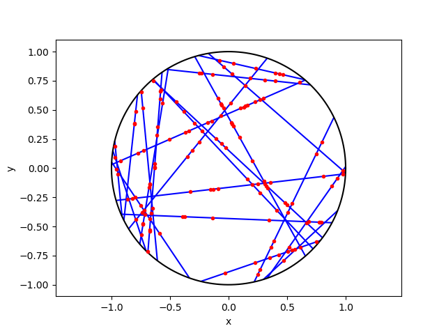
Cox-Poisson line-point process
To construct this Cox point process, we first consider a Poisson line process, which I discussed previously. Given a Poisson line process, we then place an independent one-dimensional Poisson point process on each line. We then obtain an example of a Cox point process, which we could call a Cox line-point process or a Cox-Poisson line-point process. (But I am not sure of the best name.)
Researchers have recently used this point process to study wireless communication networks in cities, where the streets correspond to Poisson lines. For example, see these two preprints:
Shot-noise Cox point process
We construct the next Cox point process by first considering a Poisson point process on the space \(\mathbb{S}\) to create a shot noise term. (Shot noise is just the sum of some function over all the points of a point process.) We then use it as the driving measure of the Cox point process.
More specifically, we first introduce a kernel function \(k(\cdot,\cdot)\) on \(\mathbb{S}\), where \(k(x,\cdot)\) is a probability density function for all points \(x\in \mathbb{S}\). We then consider a Poisson point process \(\Phi’\) on \(\mathbb{S}\times (0,\infty)\). We assume the Poisson point process \(\Phi’\) has a locally integrable intensity function \(\mu \).
(We can interpret the point process \(\Phi’\) as a spatially-dependent marked Poisson point process, where the unmarked Poisson point process is defined on \(\mathbb{S}\). We then assume each point \(X\) of this unmarked point process has a mark \(T \in (0,\infty)\) with probability density \(\mu(X,t)\).)
The resulting shot noise
$$
Z(x)= \sum_{(Y,T)\in \Phi’} T \, k(Y,x)\,,
$$
gives the random field. We then use it as the random intensity function to drive the shot-noise Cox point process.
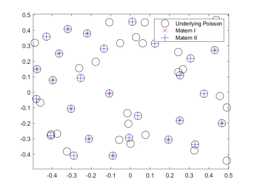
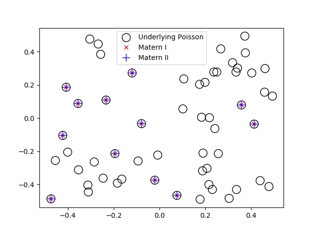
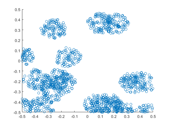
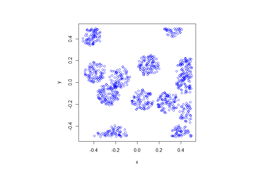
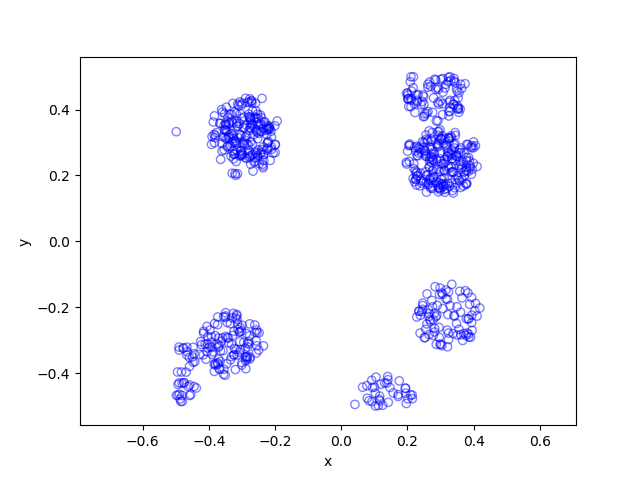
In previous posts, I have detailed how to simulate non-Poisson point processes such as the Matérn and Thomas cluster point processes. These are examples of a Neyman-Scott point process, which is a special case of a shot noise Cox point process. All these point processes find applications in spatial statistics.
Simulation
Unfortunately, there is no universal way to simulate all Cox point processes. (And even if there were one, it would not be the most optimal way for every Cox point process.) The simulation method depends on how the Cox point process is constructed, which usually means how its directing or driving measure is defined.
In previous posts I have presented ways (with code) to simulate these Cox point processes:
- Matérn (cluster) point processes (code);
- Thomas (cluster) point processes (code);
- Cox-Poisson line-point process (code).
In addition to the Matérn and Thomas point processes, there are ways to simulate more general shot noise Cox point processes. I will cover that in another post.
Further reading
For general Cox point processes, I suggest: Chapter 6 in the monograph Poisson Processes by Kingman; Chapter 5 in Statistical Inference and Simulation for Spatial Point Processes by Møller and Waagepetersen; and Section 5.2 in Stochastic Geometry and its Applications by Chiu, Stoyan, Kendall and Mecke. For a much more mathematical treatment, see Chapter 13 in Lectures on the Poisson Process by Last and Penrose. Grandell wrote two detailed monographs titled Mixed Poisson Process and Doubly Stochastic Poisson Processes.
Motivated by applications in spatial statistics, Jesper Møller has (co)-written papers on specific Cox point processes. For example:
- 2001, Møller, Syversveen, and Waagepetersen, Log Gaussian Cox Processes;
- 2003, Møller, Shot noise Cox Processes;
- 2005, Møller and Torrisi,Generalised shot noise Cox processes.
I also suggest the survey article:
- 2003, Møller and Waagepetersen, Modern statistics for spatial point processes.