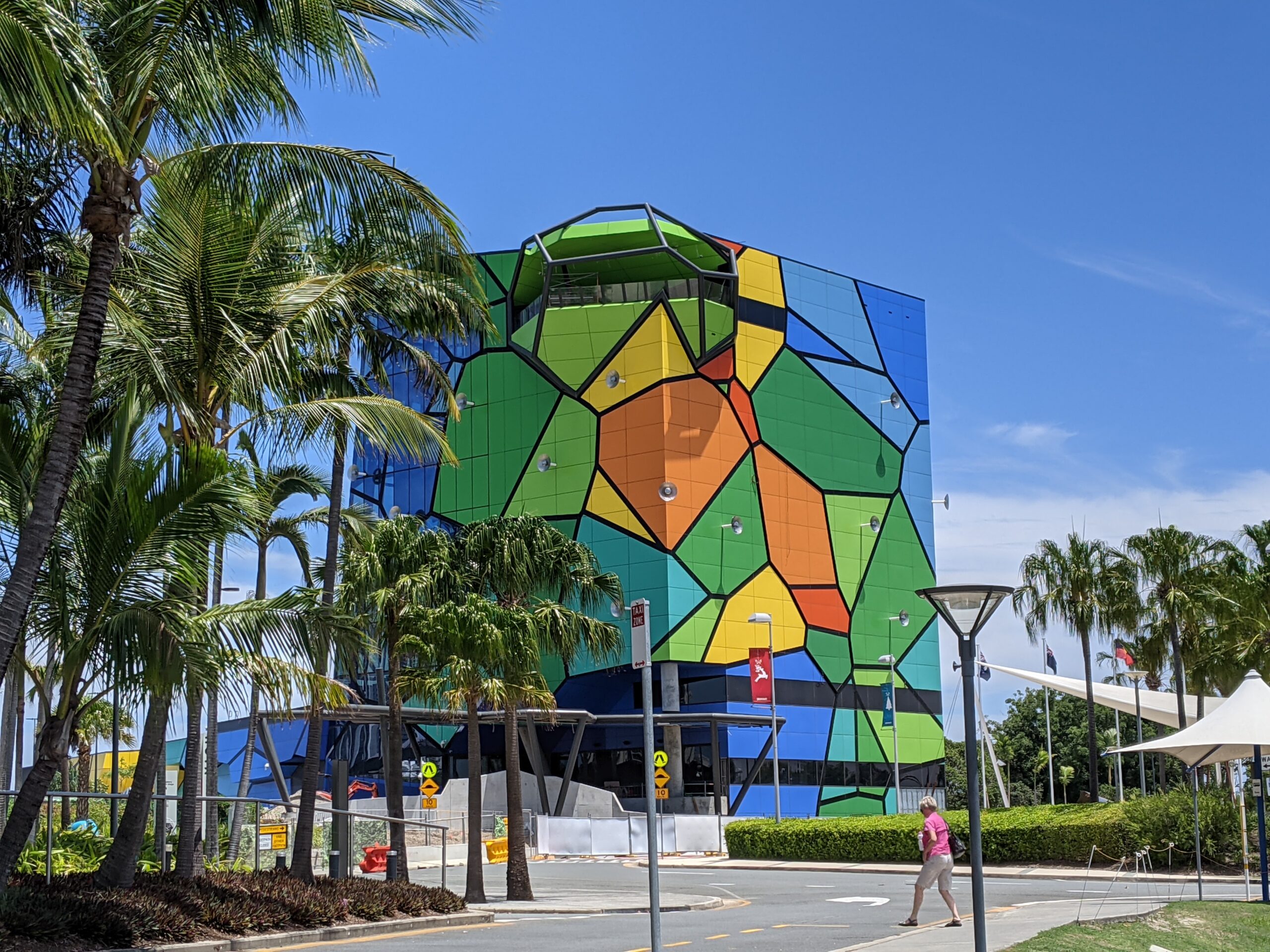
A colleague just sent me this photo of a colourful building on the Gold Coast. The building is the new Home of the Arts (HOTA) Gallery, as detailed here. It is covered in a Voronoi tessellation. I described this very useful geometrical object in a previous post.
The New HOTA Gallery with a Voronoi tessellation on the outside.
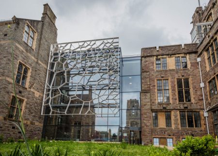
A casual Google reveals that other buildings have Voronoi-inspired architecture. For example, The Fry building at the University of Bristol in Britain, which fittingly houses the mathematics department.
The Fry Building at the University of Bristol (Source)
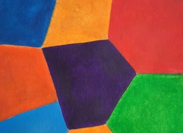
The building for the Alibaba headquarters in China also evokes Voronoi imagery. But those Voronoi constructions do no feature the colours of the HOTA Gallery, which is reminiscent of diagrams produced by scientific plotting packages.
(Of course I don’t mind the odd Voronoi tesselation. For example, a couple of months ago I set for my website image a Voronoi tesselation, created by the Franco-German artist Plaisance Puisatier. And the cover of a book I co-wrote has a diagram based on the signal-to-interference ratio, which can be considered as a generalization of a Voronoi tessellation.)
Mathematical buildings
Another building that employs an interesting geometrical object is RMIT’s Storey Hall, located in Melbourne. It features Penrose tiling, which is an example of a non-periodic tiling. Loosely speaking, that means if you tile an infinite plane with a given a set of tiles, then no translation of the plane will yield the same pattern again. The Penrose tiling is also inside the building, as you can see on this website.
On topic of non-periodic tiling, the buildings at Federation Square in Melbourne are covered by pinwheel tiling, as shown on this mathematics website, which is also non-periodic. According to Wikipedia, Charles Radin proposed this tiling based on a construction by the late and famous John Conway who died earlier this year, being yet another victim of the pandemic.
Mathematical architects
While writing this post, I noticed that both the HOTA Gallery and Storey Hall were designed by ARM Architecture. Some of their other buildings have a geometrical aspect. Clearly they have a mathematical inclination.
Cholera outbreaks due to public water pumps. Suburbs serviced by hospitals. Formation of crystals. Coverage regions of phone towers. We can model or approximate all these phenomena and many, many more with a geometric structure called, among other names, a Voronoi tessellation.
To form a Voronoi tessellation, consider a collection of points scattered on some space, like the plane, where it’s easier to picture things, especially when using a Euclidean metric. Now for each point in the collection, consider the surrounding region that is closer to that point than any other point in the collection. Each region forms a cell corresponding to the point. The union of all the sets covers the underlying space. That union of sets is the Voronoi tessellation.
The evolution of Voronoi cells, which start off as disks until they collide with each other. Source: Wikipedia.
Mathematicians have extensively studied Voronoi tessellations, particularly those based on Poisson point processes, forming a core subject in the field of stochastic geometry.
It’s also called a Dirichlet tessellation
The main other name for the Voronoi tessellation is the Dirichlet tessellation. Historically, Dirichlet beats Voronoi, but it seems wherever I look, the name Voronoi usually wins out, suggesting an example of Stigler’s law of eponymy. A notable exception is the R library spatstat that does actually call it a Dirichlet tessellation. Wikipedia calls it a Voronoi diagram. I’ve read that Descartes studied the object even earlier than Dirichlet, but Voronoi studied it in much more depth. At any rate, I will call it a Voronoi tessellation.
Everyday Voronoi tessellations
Voronoi tessellations are just not interesting mathematical objects, as they arise in everyday situations. This piece from Scientific American website explains:
Everyone uses Voronoi tessellations, even without realizing it. Individuals seeking the nearest café, urban planners determining service area for hospitals, and regional planners outlining school districts all consider Voronoi tessellations. Each café, school, or hospital is a site from which a Voronoi tessellation is generated. The cells represent ideal service areas for individual businesses, schools, or hospitals to minimize clientele transit time. Coffee drinkers, patients, or students inside a service area (that is, a cell) should live closer to their own café, hospital, or school (that is, their own cell’s site) than any other. Voronoi tessellations are ubiquitous, yet often invisible.
Delaunay triangulation
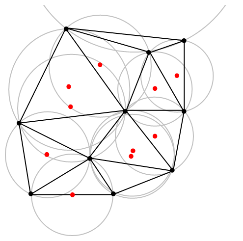
A closely related object is the Delaunay triangulation. For a given collection of points on some underlying mathematical space, a Delaunay triangulation is formed by connecting the points and creating triangles with the condition that for each point, no other point exists in the circumcircle of the corresponding triangle. (A circumcircle is a circle that passes through all three vertices of a triangle.)
An example of Delaunay triangulation with the original points in black and centrers (in red) of the corresponding circumcircles (in grey) of the Delaunay triangles. Source: Wikipedia.
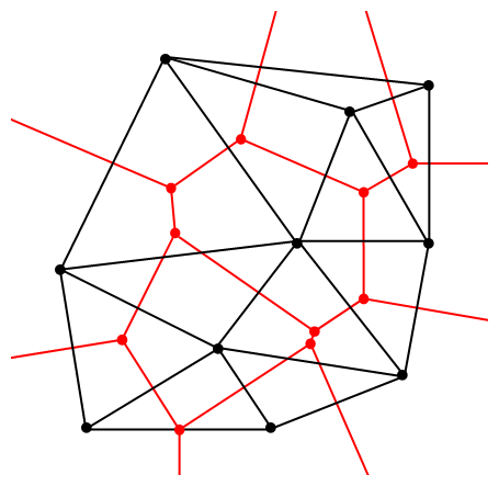
The vertices of the the Delaunay triangular and Voronoi tessellation both form graphs, which turn out to be the dual graphs of each other.
A Delaunay triangulation (in black) and the corresponding Voronoi tessellation (in red) whose vertices are the centres of the circumcircles of the Delaunay triangles. Source: Wikipedia.
Software: Qhull
Due to its applications, it’s not surprising that there exist algorithms that quickly create or estimate Voronoi tessellations. I don’t want to implement one of these algorithms from scratch, as they have already been implemented in various scientific programming languages. Many of the languages, such as MATLAB, R, and Python (SciPy) use the code from Qhull. (Note the Qhull website calls the tessellation a Voronoi diagram.)
(The Julia programming language, which I examined in a previous post, has a Voronoi package that does not use Qhull.)
Qhull finds the Voronoi tessellation by first finding the Delaunay triangulation. If the underlying space is bounded, then all the Voronoi cells are also bounded. But on an unbounded space, it is possible to have unbounded cells, meaning their areas (or volumes) are infinite. In such cases, the algorithms sometime place virtual points at infinity, but I don’t want to focus on such details. I will assume Qhull does a good job.
Code
As always, the code from all my posts is online. For this post, the MATLAB and Python code is here and here, respectively, which generates Voronoi tesselations.
MATLAB
It is fairly straightforward to create Voronoi tessellations in MATLAB. You can just use the function voronoi, which is only for two-dimensional tessellations. (Note: the MATLAB website says the behaviour of the function voronoi has changed, so that may cause problems when using different versions of MATLAB.) The function requires two inputs as vectors, say, x and y, corresponding to the Cartesian (or \(x\) and \(y\)) coordinates of the points. If you just run the voronoi command, it will create and plot a Voronoi tessellation (or Voronoi diagram, as MATLAB calls it). But the MATLAB website also describes how to plot the tessellation manually.
For \(d\) -dimensional tessellations, there is the function voronoin, which requires a single input. The single output consists of combining \(d\) column vectors for the Cartesian coordinates. For example, given the column vectors x, y and z, then the input is [x, y, z].
If you give the functions voronoi or voronoin output arguments, then the tessellation is not plotted and instead two data structures, say, v and c are created for describing the vertices of the tessellation. I generally use voronoi for plotting, but I use voronoin (and not voronoi) for generating vertex data, so I will focus on the outputs of voronoin.
For voronoin, the first (output) data structure v is simply an two-dimensional array array that contain the Cartesian coordinates of every vertex in the Voronoi tessellation. The second (output) data structure c is a cell array describing the vertices of each Voronoi cell (it has to be a cell array, as opposed to a regular array, as the cells have varying number of vertices). Each entry of the cell array contains a one-dimensional array with array indices corresponding to the \(x\) and \(y\) coordinates.
The code checks which Voronoi cells are unbounded by seeing if they have vertices at infinity, which corresponds to a \(1\) in the index arrays (stored in the structure array c).
One criticism of the MATLAB functions is that they don’t return all the information of the Voronoi tessellation. More specifically, the functions don’t return the boundaries between the unbounded cells, though voronoi internally calculates and uses these boundaries to generate Voronoi plots. This is covered in this review on different Voronoi packages. Conversely, the Python package returns more information such as that of the edges or ridges of the Voronoi cells.
Python
To create the Voronoi tessellation, use the SciPy (Spatial) function Voronoi. This function does \(d\)-dimensional tessellations. For the two-dimensional setting, you need to input the \(x\) and \(y\) coordinates as a single array of dimensions \(2 \times n\), where \(n\) is the number of points in the collection. In my code, I start off with two one-dimensional arrays for the Cartesian coordinates, but then I combined them into a single array by using the function numpy.stack with the function argument axis =1.
I would argue that the Voronoi function in SciPy is not as intuitive to use as the MATLAB version. One thing I found a bit tricky, at first, is that the cells and the points have a different sets of numbering (that is, they are indexed differently). (And I am not the only one that was caught by this.) You must use the attribute called point_region to access a cell number (or index) from a point number (or index). In my code the attribute is accessed and then called it indexP2C, which is an integer array with cell indices. Of course, there could be a reason for this, and I am just failing to understand it.
Apart from the above criticism, the function Voronoi worked well. As I mentioned before, this package returns more Voronoi information than the MATLAB equivalents.
To plot the Voronoi tessellation, use the SciPy function voronoi_plot_2d, which allows for various plotting options, but it does require Matplotlib. The input is the data object created by the function Voronoi.
Results
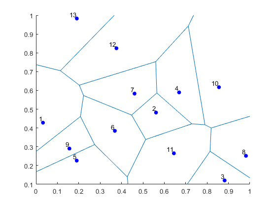
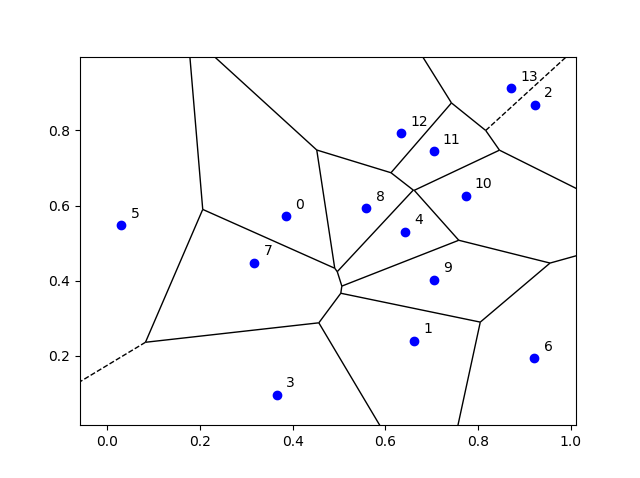
I’ve plotted the results for a single realization of a Poisson point process. I’ve also plotted the indices of the points. Recall that the indexing in Python and MATLAB start respectively at zero and one.
MATLAB
Python
Voronoi animations
I took the animation of evolving Voronoi cells, which appears in the introduction, from Wikipedia. The creator generated it in MATLAB and also posted the code online. The code is long, and I wouldn’t even dare to try to reproduce it, but I am glad someone else wrote it.
Such animations exist also for other metrics. For example, the Manhattan metric (or taxi cab or city block metric) gives the animation below, where the growing disks have been replaced with squares.
A Voronoi tessellation under the Manhattan metric. The evolving cells start off as squares until they collide with each other. Source: Wikipedia.
This Wikipedia user page has animations under other metrics on Euclidean space.
This post also features animations of Voronoi tessellations when the points move.
Further reading
There is a lot of literature on Voronoi or Dirichlet tessellations, particularly when the seeds of the cells form a Poisson point process. The references in the articles on Wikipedia and MathWorld are good starting points.
Here is a good post on Voronoi tesselations. Here is a non-mathematical article published in the Irish Times.

