Sometimes with just a little tweaking of a point process, you can get a new point process. An example of this is the Thomas point process, which is a type of cluster point process, meaning that its randomly located points tend to form random clusters. This point process is an example of a family of cluster point processes known as Neyman-Scott point processes, which have been used as models in spatial statistics and telecommunications. If that sounds familiar, that is because this point process is very similar to the Matérn point cluster process, which I covered in the previous post.
The only difference between the two point processes is how the points are randomly located. In each cluster of a Thomas point process, each individual point is located according to two independent zero-mean normal variables with variance \(\sigma^2\), describing the \(x\) and \(y\) coordinates relative to the cluster centre, whereas each point of a Matérn point process is located uniformly in a disk.
Working in polar coordinates, an equivalent way to simulate a Thomas point process is to use independent and identically-distributed Rayleigh random variables for the radial (or \(\rho\)) coordinates, instead of using random variables with a triangular distribution, which are used to simulate the Matérn point process. This method works because in polar coordinates a uniform random variable for the angular (or \(\theta\) ) coordinate and a Rayleigh random variable for the angular (or \(\rho\)) is equivalent to in Cartesian coordinates two independent zero-mean normal variables. This is exactly the trick behind the Box-Muller transform for generating normal random variables using just uniform random variables.
If you’re familiar with simulating the Matérn point process, the most difference is what size to make the simulation window for the parents points. I cover that in the next section.
Overview
Simulating a Thomas cluster point process requires first simulating a homogeneous Poisson point process with intensity \(\lambda>0\) on some simulation window, such as a rectangle, which is the simulation window I will use here. Then for each point of this underlying point process, simulate a Poisson number of points with mean \(\mu>0\), and for each point simulate two independent zero-mean normal variables with variance \(\sigma^2\), corresponding to the (relative) Cartesian coordinates .
The underlying point process is sometimes called the parent (point) process, and its points are centres of the cluster disks. The subsequent point process on all the disks is called daughter (point) process and it forms the clusters. I have already written about simulating the homogeneous Poisson point processes on a rectangle and a disk, so those posts are good starting points, and I will not focus too much on details for these steps steps.
Importantly, like the Matérn point process, it’s possible for daughter points to appear in the simulation window that come from parents points outside the simulation window. To handle these edge effects, the point processes must be first simulated on an extended version of the simulation window. Then only the daughter points within the simulation window are kept and the rest are removed.
We can add a strip of some width \(d\) all around the simulation window. But what value does \(d\) take? Well, in theory, it is possible that a daughter point comes from a parent point that is very far from the simulation window. But that probability becomes vanishingly small as the distance increases, due to the daughter points being located according to zero-mean normal random variables.
For example, if a single parent point is at a distance \(d=6 \sigma\) from the simulation, then there is about a \(1/1 000 000 000\) chance that a single daughter point will land in the simulation window. The probability is simply \(1-\Phi(6 \sigma)\), where \(\Phi\) is the cumulative distribution function of a normal variable with zero mean and standard deviation \(\sigma>0\). This is what they call a six sigma event. In my code, I set \(d=6 \sigma\), but \(d=4 \sigma\) is good enough, which is the value that the R library spatstat uses by default.
Due to this approximation, this simulation cannot be called a perfect simulation, despite the approximation being highly accurate. In practice, it will not have no measurable effect on simulation results, as the number of simulations will rarely be high enough for (hypothetical) daughter points to come from (hypothetical) parent points outside the window.
Steps
Number of points
Simulate the underlying or parent Poisson point process on the rectangle with \(N_P\) points. Then for each point, simulate a Poisson number of offspring or daughter points, where each parent point \(D_i\) number of offspring points.
Then the total number of offspring points is simply \(N=D_1+\dots +D_{P}=\sum_{i=1}^{N_P}D_i \). The random variables \(P\) and \(D_i\) are Poisson random variables with respective means \(\lambda A\) and \(\mu\), where \(A\) is the area of the rectangular simulation window. To simulate these random variables in MATLAB, use the poissrnd function. To do this in R, use the standard function rpois. In Python, we can use either functions scipy.stats.poisson or numpy.random.poisson from the SciPy or NumPy libraries.
Locations of points
The points of the parent point process are randomly positioned by using Cartesian coordinates. For a homogeneous Poisson point process, the \(x\) and \(y\) coordinates of each point are independent uniform points, which is also the case for the binomial point process, covered in an earlier post.
As mentioned in the introduction of this post, the points of all the daughter point process are randomly positioned by either using polar coordinates or Cartesian coordinates, due to the Box-Muller transform. But because we ultimately convert back to Cartesian coordinates (for example, to plot the points), we will work entirely in this coordinate system. Each point is then simply positioned with two independent zero-mean normal random variables, representing the \(x\) and \(y\) coordinates relative to the original parent point.
Shifting all the points in each cluster disk
In practice (that is, in the code), all the daughter points are simulated relative to the origin. Then for each cluster disk, all the points need to be shifted, so the origin coincides with the parent point, which completes the simulation step.
To use vectorization in the code, the coordinates of each cluster point are repeated by the number of daughters in the corresponding cluster by using the functions repelem in MATLAB, rep in R, and repeat in Python.
Code
I have implemented the simulation procedure in MATLAB, R and Python, which as usual are all very similar. The code can be downloaded here.
MATLAB
% Simulate a Thomas cluster point process on a rectangle.
% Author: H. Paul Keeler, 2018.
% Website: hpaulkeeler.com
% Repository: github.com/hpaulkeeler/posts
% For more details, see the post:
% hpaulkeeler.com/simulating-a-thomas-cluster-point-process/

%Simulation window parameters
xMin=-.5;
xMax=.5;
yMin=-.5;
yMax=.5;

%Parameters for the parent and daughter point processes
lambdaParent=10;%density of parent Poisson point process
lambdaDaughter=100;%mean number of points in each cluster
sigma=0.05;%sigma for normal variables (ie random locations) of daughters

%Extended simulation windows parameters
rExt=6*sigma; %extension parameter -- use factor of deviation
%for rExt, use factor of deviation sigma eg 5 or 6
xMinExt=xMin-rExt;
xMaxExt=xMax+rExt;
yMinExt=yMin-rExt;
yMaxExt=yMax+rExt;
%rectangle dimensions
xDeltaExt=xMaxExt-xMinExt;
yDeltaExt=yMaxExt-yMinExt;
areaTotalExt=xDeltaExt*yDeltaExt; %area of extended rectangle

%Simulate Poisson point process for the parents
numbPointsParent=poissrnd(areaTotalExt*lambdaParent,1,1);%Poisson number
%x and y coordinates of Poisson points for the parent
xxParent=xMinExt+xDeltaExt*rand(numbPointsParent,1);
yyParent=yMinExt+yDeltaExt*rand(numbPointsParent,1);

%Simulate Poisson point process for the daughters (ie final poiint process)
numbPointsDaughter=poissrnd(lambdaDaughter,numbPointsParent,1);
numbPoints=sum(numbPointsDaughter); %total number of points

%Generate the (relative) locations in Cartesian coordinates by
%simulating independent normal variables
xx0=normrnd(0,sigma,numbPoints,1);
yy0=normrnd(0,sigma,numbPoints,1);

%replicate parent points (ie centres of disks/clusters)
xx=repelem(xxParent,numbPointsDaughter);
yy=repelem(yyParent,numbPointsDaughter);
%translate points (ie parents points are the centres of cluster disks)
xx=xx(:)+xx0;
yy=yy(:)+yy0;

%thin points if outside the simulation window
booleInside=((xx>=xMin)&(xx<=xMax)&(yy>=yMin)&(yy<=yMax));
%retain points inside simulation window
xx=xx(booleInside);
yy=yy(booleInside);

%Plotting
scatter(xx,yy);
shg;
R
The R code is located here. But, of course, as I have mentioned before, simulating a spatial point processes in R is even easier with the powerful spatial statistics library spatstat. The Thomas cluster point process is simulated by using the function rThomas, but other cluster point processes, including Neyman-Scott types, are possible.
Python
Note: in previous posts I used the SciPy functions for random number generation, but now use the NumPy ones, but there is little difference, as SciPy builds off NumPy.
# Simulate a Thomas cluster process on a rectangle.
# Author: H. Paul Keeler, 2018.
# Website: hpaulkeeler.com
# Repository: github.com/hpaulkeeler/posts
# For more details, see the post:
# hpaulkeeler.com/simulating-a-thomas-cluster-point-process/

import numpy as np;  # NumPy package for arrays, random number generation, etc
import matplotlib.pyplot as plt  # For plotting

plt.close("all");  # close all figures

# Simulation window parameters
xMin = -.5;
xMax = .5;
yMin = -.5;
yMax = .5;

# Parameters for the parent and daughter point processes
lambdaParent = 10;  # density of parent Poisson point process
lambdaDaughter = 100;  # mean number of points in each cluster
sigma = 0.05;  # sigma for normal variables (ie random locations) of daughters

# Extended simulation windows parameters
rExt=6*sigma; # extension parameter
# for rExt, use factor of deviation sigma eg 5 or 6
xMinExt = xMin - rExt;
xMaxExt = xMax + rExt;
yMinExt = yMin - rExt;
yMaxExt = yMax + rExt;
# rectangle dimensions
xDeltaExt = xMaxExt - xMinExt;
yDeltaExt = yMaxExt - yMinExt;
areaTotalExt = xDeltaExt * yDeltaExt;  # area of extended rectangle

# Simulate Poisson point process for the parents
numbPointsParent = np.random.poisson(areaTotalExt * lambdaParent);# Poisson number of points
# x and y coordinates of Poisson points for the parent
xxParent = xMinExt + xDeltaExt * np.random.uniform(0, 1, numbPointsParent);
yyParent = yMinExt + yDeltaExt * np.random.uniform(0, 1, numbPointsParent);

# Simulate Poisson point process for the daughters (ie final poiint process)
numbPointsDaughter = np.random.poisson(lambdaDaughter, numbPointsParent);
numbPoints = sum(numbPointsDaughter);  # total number of points

# Generate the (relative) locations in Cartesian coordinates by
# simulating independent normal variables
xx0 = np.random.normal(0, sigma, numbPoints);  # (relative) x coordinaets
yy0 = np.random.normal(0, sigma, numbPoints);  # (relative) y coordinates

# replicate parent points (ie centres of disks/clusters)
xx = np.repeat(xxParent, numbPointsDaughter);
yy = np.repeat(yyParent, numbPointsDaughter);

# translate points (ie parents points are the centres of cluster disks)
xx = xx + xx0;
yy = yy + yy0;

# thin points if outside the simulation window
booleInside = ((xx >= xMin) & (xx <= xMax) & (yy >= yMin) & (yy <= yMax));
# retain points inside simulation window
xx = xx[booleInside];
yy = yy[booleInside];

# Plotting
plt.scatter(xx, yy, edgecolor='b', facecolor='none', alpha=0.5);
plt.xlabel("x");
plt.ylabel("y");
plt.axis('equal');
Julia
After writing this post, I later wrote the code in Julia. The code is here and my thoughts about Julia are here.
Results
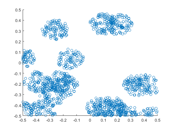
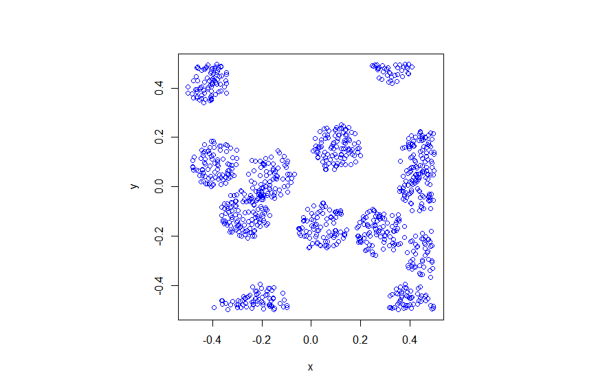
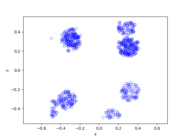
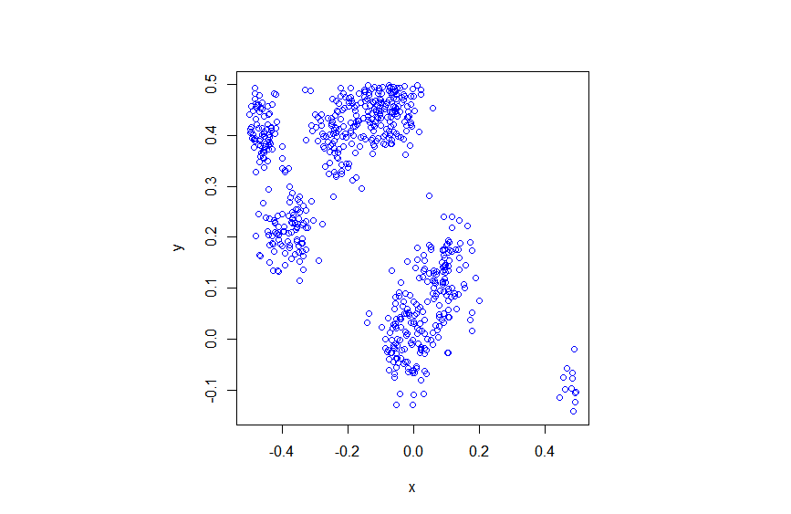
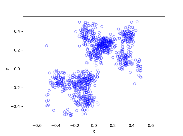
The results show that the clusters of Thomas point process tend to be more blurred than those of Matérn point process, which has cluster edges clearly defined by the disks. The points of of a Thomas point process can be far away from the centre of each cluster, depending on the variance of the normal random variables used in the simulation.
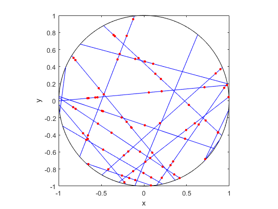
MATLAB
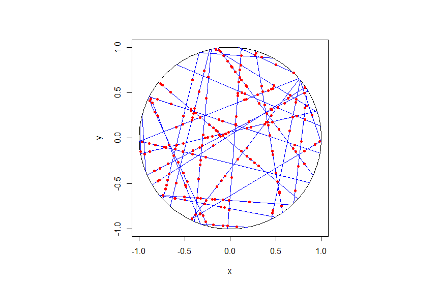
R
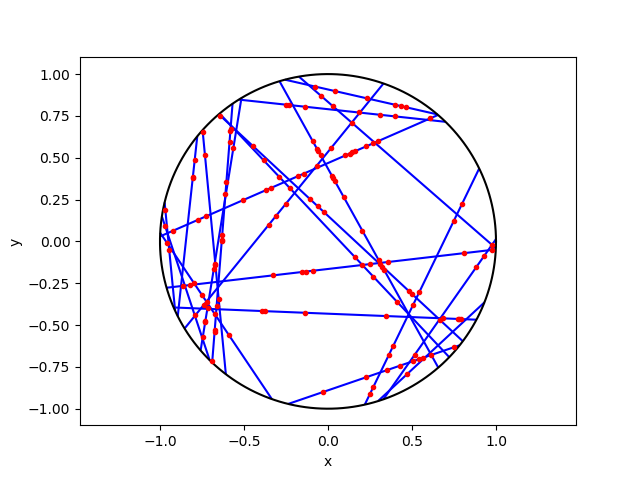
Python
Further reading
Thomas (and Matérn) cluster point processes and more generally Neyman-Scott point processes are covered in standard books on the related fields of spatial statistics, point processes and stochastic geometry, such as the following: Spatial Point Patterns: Methodology and Applications with R by Baddeley, Rubak and Turner, on page 461; Statistical Analysis and Modelling of Spatial Point Patterns Statistics by Illian, Penttinen, Stoyan, amd Stoyan, page 370 and Section 6.3.2; Stochastic Geometry and its Applications by Chiu, Stoyan, Kendall and Mecke, on page 173; and; Statistical Inference and Simulation for Spatial Point Processes by Møller and Waagepetersen, in Section 5.3. I would probably recommend the first two books for beginners.
The Thomas point process has also appeared in models of wireless networks, which we covered in the book Stochastic Geometry Analysis of Cellular Networks by Błaszczyszyn, Haenggi, Keeler, and Mukherjee, Section 8.1.8.
More generally, Neyman-Scott point processes belong to a family of point processes called shot noise Cox point processes; see the paper by Møller.
I mentioned above the book Spatial Point Patterns: Methodology and Applications with R , which is written by spatial statistics experts Baddeley, Rubak and Turner. It covers the spatial statistics (and point process simulation) R-package spatstat.
In my travels on the web, I found this post where the writer also simulates the Thomas and Matérn point processes in Python, independent of my code. That code is a bit different to mine because I use the repeat function and simulate all the Poisson variables at once, instead of using a for-loop and simulating a Poisson variable for each iteration. I also think it’s not quite correct because I do not see how they account for edge effects.