Thinning point processes

One way to create new point processes is to apply thinning to a point process. As I mentioned in a previous post on point process operations, thinning is a random operation applied to the points of an underlying point process, where the points are thinned (or removed) or retained (or kept) according to some probabilistic rule. Both the thinned and retained points form two separate point processes, but one usually focuses on the retained points. Given an underlying point process, the nature of the thinning rule will result in different types of point processes.

As I detailed in the Applications section below, thinning can be used to simulate an inhomogeneous Poisson point process, as I covered in another post.

Thinning types

Thinning can be statistically independent or dependent, meaning that the probability of thinning any point is either independent or dependent of thinning other points. The more tractable case is statistically independent thinning, which is the thinning type covered here. We can further group this thinning into two types based on whether the thinning rule depends on the locations of the point. (I use the word location, instead of point, to refer to where a point of a point process is located on the underlying mathematical space on which the point process is defined.)

Spatially independent thinning

The simplest thinning operation is one that does not depend on point locations. This thinning is sometimes referred to as \(p\)-thinning, where the constant \(p\) has the condition \(0\leq p \leq 1\) because it is the probability of thinning a single point. Simply put, the probability of a point being thinned does not depend on the point locations.

Example

We can liken the thinning action to flipping a biased coin with probability of \(p\) for heads (or tails) for each point of the underlying point process, and then removing the point if a head (or tails) occurs. If there were a constant number \(n\) of points of the underlying point process, then the number of thinned (or retained) points will form a binomial random variable with parameters \(n\) and \(p\) (or \(1-p\)).

Simulation

Simulating this thinning operation is rather straightforward. Given a realization of a point process, for each point, simply generate or simulate a uniform random variable on the interval \((0,1)\), and if this random variable is less than \(p\), remove the point. (This is simply sampling a Bernoulli distribution, which is covered in this post.)

In the code section below, I have shown how this thinning operation is implemented.

Spatially dependent thinning

To generalize the idea of \(p\)-thinning, we can simply require that the thinning probability of any point depends on its location \(x\), which gives us the concept of \(p(x)\)-thinning. (I write a single \(x\) to denote a point on the plane, that is \(x\in \mathbb{R}^2\), instead of writing, for example, the \(x\) and \(y\) and coordinates separately.) More precisely, the probability of thinning a point is given by a function \(p(x)\) such that \(0 \leq p(x)\leq 1\), but all point thinnings occur independently of each other. In other words, this is a spatially dependent thinning that is statistically independent.

Example

I’ll illustrate the concept of (statistically independent) spatially dependent thinning with a somewhat contrived example. We assume that the living locations of all the people in the world form a point process on a (slightly squashed) sphere. Let’s say that Earth has become overpopulated, particularly in the Northern Hemisphere, so we decide to randomly choose people and send them off to another galaxy, but we do it based on how far they live from the North Pole. The thinning rule could be, for example, \(p(x)= \exp(- |x|^2/s^2)\), where \(|x|\) is the distance to the North Pole and \(s>0\) is some constant for distance scaling.

Put another way, a person at location \(x\) flips a biased coin with the probability of heads being equal to \(p(x)=\exp(- |x|^2/s^2)\). If a head comes up, then that person is removed from the planet. With the maximum of \(p(x)\) is at the North Pole, we can see that the lucky (or unlucky?) people in countries like Australia, New Zealand (or Aotearoa), South Africa, Argentina and Chile, are more likely not to be sent off (that is, thinned) into the great unknown.

For people who live comparable distances from the North Pole, the removal probabilities are similar in value, yet the events of being remove remain independent. For example, the probabilities of removing any two people from the small nation Lesotho are similar in value, but these two random events are still completely independent of each other.

Simulation

Simulating a spatially dependent thinning is just slightly more involved than the spatially independent case. Given a realization of a point process, for each point at, say, \(x\), simply generate or simulate a uniform random variable on the interval \((0,1)\), and if this random variable is less than \(p(x)\), remove the point.

In the code section, I have shown how this thinning operation is implemented with an example like the above one, but on a rectangular region of Cartesian space. In this setting, the maximum of \(p(x)\) is at the origin, resulting in more points being thinned in this region.

Thinning a Poisson point process

Perhaps not surprisingly, under the thinning operation the Poisson point process exhibits a closure property, meaning that a Poisson point process thinned in a certain way gives another Poisson point process.  More precisely, if the thinning operation is statistically independent, then the resulting point process formed from the retained points is also a Poisson point process, regardless if it is spatially independent or dependent thinning. The resulting intensity (interpreted as the average density of points) of this new Poisson point process has a simple expression.

Homogeneous case

For a spatially independent \(p\)-thinning, if the original (or underlying) Poisson point process is homogeneous with intensity \(\lambda\), then the point process formed from the retained points is a homogeneous Poisson point process with intensity \(\lambda\).  (There are different ways to prove this, but you can gain some intuition behind the proof by conditioning on the Poisson number of points and then applying the total law of probability. Using generating functions helps.)

Inhomogeneous case

More generally, if we apply a spatially dependent \(p(x)\)-thinning to a  Poisson point process has a intensity \(\lambda\), then the retained points form a  an inhomogeneous or nonhomogeneous Poisson point process with \(\lambda p(x)\),  due to the spatial dependence in the thinning function \(p(x)\). This gives a way to simulate such Poisson point processes, which I’ll cover in another post.

Splitting

We can see by symmetry that if we look at the thinned points, then the resulting point process is also a Poisson point process, but with intensity \((1-p(x))\lambda\). The retained and thinned points both form Poisson point processes, but what is really interesting is these two point processes are independent of each other.  This means that any random configuration that occurs among the retained points is independent of any configurations among the thinned points.

This ability to split a Poisson point processes into independent ones is sometimes called the splitting property.

Applications

Thinning point processes has the immediate application of creating new point processes. It can also be used to randomly generate two point processes from one. In network applications, a simple example is using the thinning procedure to model random sleep schemes in wireless networks, where random subsets of the network have been powered down.

Perhaps the most useful application of thinning is creating point processes with spatially-dependent intensities such that of an inhomogeneous Poisson point process. In another post I give details on how to simulate this point process.  In this setting, the thinning operation essentially is acceptance(-rejection) sampling, which I will cover in a future post.

Code

All code from my posts, as always, can be found on the my GitHub repository. The code for this post is located here.

Spatially independent thinning

I have implemented in code the simple \(p\)-thinning operation applied to a Poisson point process on a rectangle, but in theory any point process can be used for the underlying point process that is thinned.

MATLAB

%Simulation window parameters
xMin=-1;xMax=1;
yMin=-1;yMax=1;
xDelta=xMax-xMin;yDelta=yMax-yMin; %rectangle dimensions
areaTotal=xDelta*yDelta; %area of rectangle

%Point process parameters
lambda=100; %intensity (ie mean density) of the Poisson process

%Thinning probability parameters
sigma=1;
p=0.25; %thinning probability

%Simulate Poisson point process
numbPoints=poissrnd(areaTotal*lambda);%Poisson number of points
xx=xDelta*(rand(numbPoints,1))+xMin;%x coordinates of Poisson points
yy=xDelta*(rand(numbPoints,1))+yMin;%y coordinates of Poisson points

%Generate Bernoulli variables (ie coin flips) for thinning
booleThinned=rand(numbPoints,1)>p; %points to be thinned
booleRetained=~booleThinned; %points to be retained

%x/y locations of thinned points
xxThinned=xx(booleThinned); yyThinned=yy(booleThinned);
%x/y locations of retained points
xxRetained=xx(booleRetained); yyRetained=yy(booleRetained);

%Plotting
plot(xxRetained,yyRetained,'bo'); %plot retained points
hold on; plot(xxThinned,yyThinned,'ro'); %plot thinned points
xlabel('x');ylabel('y');

R

#Simulation window parameters
xMin=-1;xMax=1;
yMin=-1;yMax=1;
xDelta=xMax-xMin;yDelta=yMax-yMin; #rectangle dimensions
areaTotal=xDelta*yDelta;

#Point process parameters
lambda=100; #intensity (ie mean density) of the Poisson process

#Thinning probability
p=0.25; 

#Simulate a Poisson point process
numbPoints=rpois(1,areaTotal*lambda);#Poisson number of points
xx=xDelta*runif(numbPoints)+xMin;#x coordinates of Poisson points
yy=xDelta*runif(numbPoints)+yMin;#y coordinates of Poisson points

#Generate Bernoulli variables (ie coin flips) for thinning
booleThinned=runif(numbPoints)>p; #points to be thinned
booleRetained=!booleThinned; #points to be retained

#x/y locations of thinned points
xxThinned=xx[booleThinned]; yyThinned=yy[booleThinned];
#x/y locations of retained points
xxRetained=xx[booleRetained]; yyRetained=yy[booleRetained];

#Plotting
par(pty="s")
plot(xxRetained,yyRetained,'p',xlab='x',ylab='y',col='blue'); #plot retained points
points(xxThinned,yyThinned,col='red'); #plot thinned points

Of course, as I have mentioned before, simulating a spatial point processes in R is even easier with the powerful spatial statistics library spatstat.  With this library, thinning can be done in quite a general way by using the function rthin.

Python

import numpy as np; #NumPy package for arrays, random number generation, etc
import matplotlib.pyplot as plt

#Simulation window parameters
xMin=-1;xMax=1;
yMin=-1;yMax=1;
xDelta=xMax-xMin;yDelta=yMax-yMin; #rectangle dimensions
areaTotal=xDelta*yDelta;

#Point process parameters
lambda0=100; #intensity (ie mean density) of the Poisson process

#Thinning probability
p=0.25; 

#Simulate a Poisson point process
numbPoints = np.random.poisson(lambda0*areaTotal);#Poisson number of points
xx = np.random.uniform(0,xDelta,((numbPoints,1)))+xMin;#x coordinates of Poisson points
yy = np.random.uniform(0,yDelta,((numbPoints,1)))+yMin;#y coordinates of Poisson points

#Generate Bernoulli variables (ie coin flips) for thinning
booleThinned=np.random.uniform(0,1,((numbPoints,1)))>p; #points to be thinned
booleRetained=~booleThinned; #points to be retained

#x/y locations of thinned points
xxThinned=xx[booleThinned]; yyThinned=yy[booleThinned];
#x/y locations of retained points
xxRetained=xx[booleRetained]; yyRetained=yy[booleRetained];

#Plotting
plt.scatter(xxRetained,yyRetained, edgecolor='b', facecolor='none', alpha=0.5 );
plt.scatter(xxThinned,yyThinned, edgecolor='r', facecolor='none', alpha=0.5 );
plt.xlabel("x"); plt.ylabel("y");
plt.show(); 

Spatially dependent thinning

I have implemented in code a \(p(x)\)-thinning operation with the function \(p(x)=\exp(-|x|^2/s^2)\), where \(|x|\) is the Euclidean distance from \(x\) to the origin. This small changes means that in the code there will be a vector or array of \(p\) values instead of a single \(p\) value in the section where the uniform random variables are generated and compared said \(p\) values.  (Lines 24, 26 and 28 respectively in the MATLAB, R and Python code presented below.)

Again, I have applied thinning to a Poisson point process on a rectangle, but in theory any point process can be used for the underlying point process.

MATLAB

%Simulation window parameters
xMin=-1;xMax=1;
yMin=-1;yMax=1;
xDelta=xMax-xMin;yDelta=yMax-yMin; %rectangle dimensions
areaTotal=xDelta*yDelta; %area of rectangle
 
%Point process parameters
lambda=100; %intensity (ie mean density) of the Poisson process

%Thinning probability parameters
sigma=0.5; %scale parameter for thinning probability function
%define thinning probability function
fun_p=@(s,x,y)(exp(-(x.^2+y.^2)/s^2)); 

%Simulate Poisson point process
numbPoints=poissrnd(areaTotal*lambda);%Poisson number of points
xx=xDelta*(rand(numbPoints,1))+xMin;%x coordinates of Poisson points
yy=xDelta*(rand(numbPoints,1))+yMin;%y coordinates of Poisson points

%calculate spatially-dependent thinning probabilities
p=fun_p(sigma,xx,yy); 

%Generate Bernoulli variables (ie coin flips) for thinning
booleThinned=rand(numbPoints,1)>p; %points to be thinned
booleRetained=~booleThinned; %points to be retained

%x/y locations of thinned points
xxThinned=xx(booleThinned); yyThinned=yy(booleThinned);
%x/y locations of retained points
xxRetained=xx(booleRetained); yyRetained=yy(booleRetained);

%Plotting
plot(xxRetained,yyRetained,'bo'); %plot retained points
hold on; plot(xxThinned,yyThinned,'ro'); %plot thinned points
xlabel('x');ylabel('y');

R

#Simulation window parameters
xMin=-1;xMax=1;
yMin=-1;yMax=1;
xDelta=xMax-xMin;yDelta=yMax-yMin; #rectangle dimensions
areaTotal=xDelta*yDelta;

#Point process parameters
lambda=100; #intensity (ie mean density) of the Poisson process

#Thinning probability parameters
sigma=0.5; #scale parameter for thinning probability function
#define thinning probability function
fun_p <- function(s,x,y) {
  exp(-(x^2 + y^2)/s^2);
}

#Simulate a Poisson point process
numbPoints=rpois(1,areaTotal*lambda);#Poisson number of points
xx=xDelta*runif(numbPoints)+xMin;#x coordinates of Poisson points
yy=xDelta*runif(numbPoints)+yMin;#y coordinates of Poisson points

#calculate spatially-dependent thinning probabilities
p=fun_p(sigma,xx,yy); 

#Generate Bernoulli variables (ie coin flips) for thinning
booleThinned=runif(numbPoints)<p; #points to be thinned
booleRetained=!booleThinned; #points to be retained

#x/y locations of thinned points
xxThinned=xx[booleThinned]; yyThinned=yy[booleThinned];
#x/y locations of retained points
xxRetained=xx[booleRetained]; yyRetained=yy[booleRetained];

#Plotting
par(pty="s")
plot(xxRetained,yyRetained,'p',xlab='x',ylab='y',col='blue'); #plot retained points
points(xxThinned,yyThinned,col='red'); #plot thinned points

Again, use the spatial statistics library spatstat, which has the function rthin.

Python

import numpy as np; #NumPy package for arrays, random number generation, etc
import matplotlib.pyplot as plt

#Simulation window parameters
xMin=-1;xMax=1;
yMin=-1;yMax=1;
xDelta=xMax-xMin;yDelta=yMax-yMin; #rectangle dimensions
areaTotal=xDelta*yDelta;

#Point process parameters
lambda0=100; #intensity (ie mean density) of the Poisson process

#Thinning probability parameters
sigma=0.5; #scale parameter for thinning probability function
#define thinning probability function
def fun_p(s, x, y):
    return np.exp(-(x**2+y**2)/s**2);    

#Simulate a Poisson point process
numbPoints = np.random.poisson(lambda0*areaTotal);#Poisson number of points
xx = np.random.uniform(0,xDelta,((numbPoints,1)))+xMin;#x coordinates of Poisson points
yy = np.random.uniform(0,yDelta,((numbPoints,1)))+yMin;#y coordinates of Poisson points

#calculate spatially-dependent thinning probabilities
p=fun_p(sigma,xx,yy); 

#Generate Bernoulli variables (ie coin flips) for thinning
booleThinned=np.random.uniform(0,1,((numbPoints,1)))>p; #points to be thinned
booleRetained=~booleThinned; #points to be retained

#x/y locations of thinned points
xxThinned=xx[booleThinned]; yyThinned=yy[booleThinned];
#x/y locations of retained points
xxRetained=xx[booleRetained]; yyRetained=yy[booleRetained];

#Plotting
plt.scatter(xxRetained,yyRetained, edgecolor='b', facecolor='none', alpha=0.5 );
plt.scatter(xxThinned,yyThinned, edgecolor='r', facecolor='none', alpha=0.5 );
plt.xlabel("x"); plt.ylabel("y");
plt.show(); 

Results

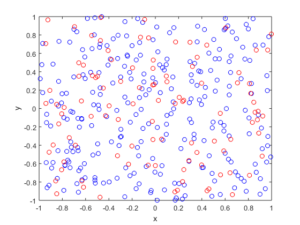
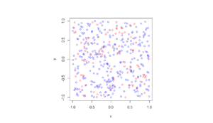
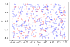
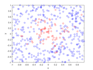
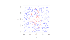
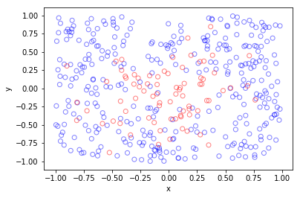
In the plotted results, the blue and red circles represent respectively the retained and thinned points.

Spatially independent thinning

For these results, I used a thinning probability \(p=0.25\), which means that roughly a quarter of the points will be thinned, so on average the ratio of blue to red circles is three to one.

MATLAB

R

Python

Spatially dependent thinning

Observe how there are more thinned points (that is, red circles) near the origin, which is of course where the thinning function \(p(x)=\exp(-|x|^2/s^2)\) attains its maximum.

MATLAB

R

Python

Further reading

The thinning operation is covered in Stochastic Geometry and its Applications by Chiu, Stoyan, Kendall and Mecke (Chapter 5). It is also covered in the book Statistical Inference and Simulation for Spatial Point Processes by Moller and Waagepetersen (Section 3.2.2). Kallenberg presents a more theoretical and rigorous take on thinning Poisson point processes in his new book Random Measures, Theory and Applications (Chapter 3). (A point process can be interpreted as a type of random measure called a random counting measure because it gives the random number of points in a set.)

Thinning is also covered in books that apply point processes to wireless networks, such as Stochastic Geometry and Wireless Networks by Baccelli and Błaszczyszyn (Volume 1, Section 1.3.2) or Stochastic Geometry for Wireless Networks (Section 2.7.3) by Haenggi. These books also give examples of thinning point processes for wireless network applications.