August 2018 – H. Paul Keeler

This is the first of a series of posts about simulating Poisson point processes. I’ll start with arguably the simplest Poisson point process on two-dimensional space, which is the homogeneous one defined on a rectangle. Let’s say that we we want to simulate a Poisson point process with intensity $\lambda>0$ on a (bounded) rectangular region, for example, the rectangle $[0,w]\times[0,h]$ with dimensions $w>0$ and $h>0$ and area $A=wh$. We assume for now that the bottom left corner of the rectangle is at the origin.

Steps

Number of points

The number of points in the rectangle $[0,w]\times[0,h]$ is a Poisson random variable with mean $\lambda A$. In other words, this random variable is distributed according to the Poisson distribution with parameter $\lambda A$, and not just $\lambda$, because the number of points depends on the size of the simulation region.

This is the most complicated part of the simulation procedure. As long as your preferred programming language can produce (pseudo-)random numbers according to a Poisson distribution, you can simulate a homogeneous Poisson point process. There’s a couple of different ways used to simulate Poisson random variables, but we will skip the details. In MATLAB, it is done by using the poissrnd function with the argument $\lambda A$. In R, it is done similarly with the standard function rpois . In Python, we can use either the scipy.stats.poisson or numpy.random.poisson function from the SciPy or NumPy libraries.

Location of points

The points now need to be positioned randomly, which is done by using Cartesian coordinates. For a homogeneous Poisson point process, the $x$ and $y$ coordinates of each point are independent uniform points, which is also the case for the binomial point process, covered in a previous post. For the rectangle $[0,w]\times[0,h]$, the $x$ coordinates are uniformly sampled on the interval $[0,w]$, and similarly for the $y$ coordinates. If the bottom left corner of rectangle is located at the point $(x_0,y_0)$, then we just have to shift the random $x$ and $y$ coordinates by respectively adding $x_0$ and $y_0$.

Every scientific programming language has a random uniform number generator because it is the default random number generator. In MATLAB, R and SciPy, it is respectively rand, runif and scipy.stats.uniform.

Code

Here is some code that I wrote for simulating a homogeneous Poisson point process on a rectangle. You will notice that in all the code samples the part that simulates the Poisson point process requires only three lines of code: one line for the number of points and two lines lines for the $x$ and $y$ coordinates of the points.

MATLAB

%Simulation window parameters
xMin=0;xMax=1;
yMin=0;yMax=1;
xDelta=xMax-xMin;yDelta=yMax-yMin; %rectangle dimensions
areaTotal=xDelta*yDelta;

%Point process parameters
lambda=100; %intensity (ie mean density) of the Poisson process

%Simulate Poisson point process
numbPoints=poissrnd(areaTotal*lambda);%Poisson number of points
xx=xDelta*(rand(numbPoints,1))+xMin;%x coordinates of Poisson points
yy=yDelta*(rand(numbPoints,1))+yMin;%y coordinates of Poisson points

%Plotting
scatter(xx,yy);
xlabel('x');ylabel('y');

R

Note: it is a bit tricky to write “<-” in the R code (as it automatically changes to the html equivalent in the HTML editor I am using), so I have usually used “=” instead of the usual “<-”.

#Simulation window parameters
xMin=0;xMax=1;
yMin=0;yMax=1;
xDelta=xMax-xMin;yDelta=yMax-yMin; #rectangle dimensions
areaTotal=xDelta*yDelta;

#Point process parameters
lambda=100; #intensity (ie mean density) of the Poisson process

#Simulate Poisson point process
numbPoints=rpois(1,areaTotal*lambda);#Poisson number of points
xx=xDelta*runif(numbPoints)+xMin;#x coordinates of Poisson points
yy=yDelta*runif(numbPoints)+yMin;#y coordinates of Poisson points

#Plotting
plot(xx,yy,'p',xlab='x',ylab='y',col='blue');

Python

Note: “lambda” is a reserved word in Python (and other languages), so I have used “lambda0” instead.

import numpy as np
import scipy.stats
import matplotlib.pyplot as plt

#Simulation window parameters
xMin=0;xMax=1;
yMin=0;yMax=1;
xDelta=xMax-xMin;yDelta=yMax-yMin; #rectangle dimensions
areaTotal=xDelta*yDelta;

#Point process parameters
lambda0=100; #intensity (ie mean density) of the Poisson process

#Simulate Poisson point process
numbPoints = scipy.stats.poisson( lambda0*areaTotal ).rvs()#Poisson number of points
xx = xDelta*scipy.stats.uniform.rvs(0,1,((numbPoints,1)))+xMin#x coordinates of Poisson points
yy = yDelta*scipy.stats.uniform.rvs(0,1,((numbPoints,1)))+yMin#y coordinates of Poisson points
#Plotting
plt.scatter(xx,yy, edgecolor='b', facecolor='none', alpha=0.5 )
plt.xlabel("x"); plt.ylabel("y")

Julia

After writing this post, I later wrote the code in Julia. The code is here and my thoughts about Julia are here.

Results

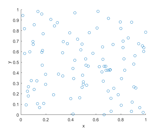
MATLAB

PoissonMatlab

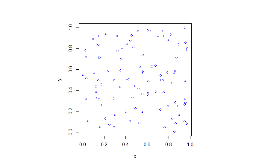
R

PoissonR

Python

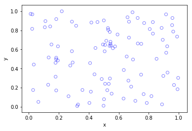
PoissonPython

Higher dimensions

If you want to simulate a Poisson point process in a three-dimensional box (typically called a cuboid or rectangular prism), you just need two modifications.

For a box $[0,w]\times[0,h]\times[0,\ell]$, the number of points now a Poisson random variable with mean $\lambda V$, where $V= wh\ell$ is the volume of the box. (For higher dimensions, you need to use $n$-dimensional volume.)

To position the points in the box, you just need an additional uniform variable for the extra coordinate. In other words, the $x$, $y$ and $z$ coordinates are uniformly and independently sampled on the respective intervals $[0,w]$, $[0,h]$, $[0,\ell]$. The more dimensions, the more uniform random variables.

And that’s it.

Month: August 2018

Simulating a homogeneous Poisson point process on a rectangle

Steps

Number of points

Location of points

Code

MATLAB

R

Python

Julia

Results

MATLAB

R

Python

Higher dimensions

Further reading