Checking Poisson point process simulations

In previous posts I described how to simulate homogeneous Poisson point processes on a rectangle, disk and triangle. Then I covered how to randomly thin a point process in a spatially dependent manner. Building off these posts, I wrote in my last post how to simulate an inhomogeneous or nonhomogeneous Poisson point process. Now I’ll describe how to verify that the simulation code correctly simulates the desired Poisson point process.

Although this post is focused on the Poisson point process, I stress that parts of the material hold for all point processes. Also, not surprisingly, some of the material and the code overlaps with that presented in the post on the inhomogeneous point process.

Basics

Any Poisson point process is defined with a measure called the intensity measure or mean measure, which I’ll denote by \(\Lambda\). For practical purposes, I assume that the intensity measure \(\Lambda\) has a derivative \(\lambda(x,y)\), where \(x\) and \(y\) denote the Cartesian coordinates. The function \(\lambda(x,y)\) is often called the intensity function or just intensity. I assume this function is bounded, so \(\lambda(x,y)<\infty\) for all points in a simulation window \(W\). Finally, I assume that the simulation window \(W\) is a rectangle.

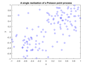
Several times before I have mentioned that simulating a Poisson point process requires simulating two random components: the number of points and the locations of points. Working backwards, to check a Poisson simulation, we must run the Poisson simulation a large number of times (say \(10^3\) or \(10^4\)), and collect the statistics on these two properties. We’ll start by examining the easiest of the two random components.

Number of points

For any Poisson point process, the number of points is a Poisson random variable with a parameter (that is, a mean) \(\Lambda(W)\). Under our previous assumptions, this is given by the surface integral

$$\Lambda(W)=\int_W \lambda(x,y)dxdy.$$

Presumably we can evaluate such an integral analytically or numerically in order to simulate the Poisson point process. To check that we correctly simulate the random the number of points, we just need to simulate the point process a large number of times, and compare the statistics to those given by the analytic expressions.

Moments

The definition of the intensity measure of a point process is a measure that gives the average or expected number of points in some region. As the number of simulations increases, the (sample) average number of points will converge to the intensity measure \(\Lambda(W)\). I should stress that this is a test for the intensity measure, a type of first moment, which will work for the intensity measure of any point process.

For Poisson point processes, there is another moment test that can be done. It can be shown mathematically that the variance of the number of points will also converge to the intensity measure \(\Lambda(W)\), giving a second empirical test based on second moments. There is no point process theory here, as this moment result is simply due to the number of points being distributed according to a Poisson distribution. The second moment is very good for checking Poissonness, forming the basis for statistical tests. If this and the first moment test hold, then there’s a very strong chance the number of points is a Poisson variable.

Empirical distribution

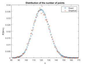
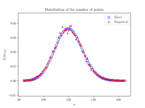
Beyond the first two moments, an even more thorough test is to estimate an empirical distribution for the number of points. That is, we perform a histogram on the number of points, and then we normalize it, so the total mass sums to one, producing an empirical probability distribution for the number of points.

The results should closely match the probability mass function of a Poisson distribution with parameter \(\Lambda(W)\). This is simply

$$ P(N=n)= \frac{[\Lambda(W)]^n}{n!} e^{-\Lambda(W)}, $$

where \(N\) is the random number of points in the window \(W\), which has the area \(|W|\). If the empirical distribution is close to results given by the above expression, then we can confidently say that the number of points is a Poisson random variable with the right parameter or mean.

Locations of points

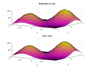
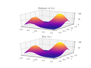
To check the positioning of points, we can empirically estimate the intensity function \(\lambda(x,y)\). A simple way to do this is to perform a two-dimensional histogram on the point locations. This is very similar to the one-dimensional histogram, which I suggested to do for testing the number of points. It just involves counting the number of points that fall into two-dimensional non-overlapping subsets called bins.

To estimate the intensity function, each bin count needs to be rescaled by the area of the bin, giving a density value for each bin. This empirical estimate of the intensity function should resemble the true intensity function \(\lambda(x,y)\). For a visual comparison, we can use a surface plot to illustrate the two sets of results.

This procedure will work for estimating the intensity function of any point process, not just a Poisson one.

Advanced tests

In spatial statistics there are more advanced statistical tests for testing how Poisson a point pattern is. But these tests are arguably too complicated for checking a simple point process that is rather easy to simulate. Furthermore, researchers usually apply these tests to a small number of point patterns. In this setting, it is not possible to accurately obtain empirical distributions without further assumptions. But with simulations, we can generate many simulations and obtain good empirical distributions. In short, I would not use such tests for just checking that I have properly coded a Poisson simulation.

Results

I produced the results with ten thousand simulations, which gave good results and took only a few seconds to complete on a standard desktop computer. Clearly increasing the number of simulations increases the accuracy of the statistics, but it also increases the computation time.

For the results, I used the intensity function

$$\lambda(x,y)=\lambda_1(x,y)+\lambda_2(x,y),$$

where

$$\lambda_1(x,y)=80e^{-((x+0.5)^2+(y+0.5)^2)/s^2},$$

$$\lambda_2(x,y)=100e^{-((x-0.5)^2+(y-0.5)^2)/s^2},$$

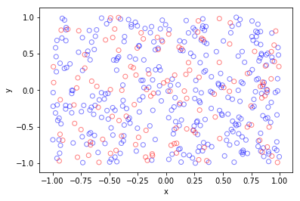
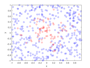
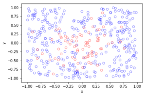
and \(s>0\) is a scale parameter. We can see that this function has two maxima or peaks at \((-0.5,-0.5)\) and \((0.5,0.5)\).

MATLAB

Python

Further reading

I have not covered much new theoretical stuff in this post, so looking at the references in previous posts, such as this one, should help.

For two-dimensional histograms, I recommend going to the respective MATLAB and Python function websites. Here’s an example of a two-dimensional histogram implemented in Python.

Probably the most difficult part for me was performing the plotting in Python. I recommend these links:

https://plot.ly/python/3d-surface-plots/

https://chrisalbon.com/python/basics/set_the_color_of_a_matplotlib/

https://matplotlib.org/examples/color/colormaps_reference.html

Code

All code from my posts, as always, can be found on the my GitHub repository. The code for this post is located here.

The estimating the statistical moments is standard. Performing the histograms is also routine, but when normalizing, you have to choose the option that returns the empirical estimate of the probability density function (pdf).

Fortunately, scientific programming languages usually have functions for performing two-dimensional histograms. What is a bit tricky is how to normalize or rescale the bin counts. The histogram functions can, for example, divide by the number of simulations, the area of each bin, or both. In the end, I chose the pdf option in both MATLAB and Python to give an empirical estimate of the probability density function, and then multiplied it by the average number of points, which was calculated in the previous check. (Although, I could have done this in a single step in MATLAB, but not in Python, so I chose to do it in a couple of steps in both languages so the code matches more closely.)

MATLAB

I used the surf function to plot the intensity function and its estimate; see below for details on the histograms.

close all;

%Simulation window parameters
xMin=-1;xMax=1;
yMin=-1;yMax=1;
xDelta=xMax-xMin;yDelta=yMax-yMin; %rectangle dimensions
areaTotal=xDelta*yDelta; %area of rectangle

numbSim=10^4; %number of simulations

s=0.5; %scale parameter

%Point process parameters
fun_lambda=@(x,y)(100*exp(-((x).^2+(y).^2)/s^2));%intensity function

%%%START -- find maximum lambda -- START %%%
%For an intensity function lambda, given by function fun_lambda,
%finds the maximum of lambda in a rectangular region given by
%[xMin,xMax,yMin,yMax].
funNeg=@(x)(-fun_lambda(x(1),x(2))); %negative of lambda
%initial value(ie centre)
xy0=[(xMin+xMax)/2,(yMin+yMax)/2];%initial value(ie centre)
%Set up optimization step
options=optimoptions('fmincon','Display','off');
%Find largest lambda value
[~,lambdaNegMin]=fmincon(funNeg,xy0,[],[],[],[],...
[xMin,yMin],[xMax,yMax],'',options);
lambdaMax=-lambdaNegMin;
%%%END -- find maximum lambda -- END%%%

%define thinning probability function
fun_p=@(x,y)(fun_lambda(x,y)/lambdaMax);

%for collecting statistics -- set numbSim=1 for one simulation
numbPointsRetained=zeros(numbSim,1); %vector to record number of points
for ii=1:numbSim
%Simulate Poisson point process
numbPoints=poissrnd(areaTotal*lambdaMax);%Poisson number of points
xx=xDelta*(rand(numbPoints,1))+xMin;%x coordinates of Poisson points
yy=xDelta*(rand(numbPoints,1))+yMin;%y coordinates of Poisson points

%calculate spatially-dependent thinning probabilities
p=fun_p(xx,yy);

%Generate Bernoulli variables (ie coin flips) for thinning
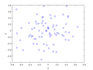
booleRetained=rand(numbPoints,1)<p; %points to be retained %x/y locations of retained points xxRetained=xx(booleRetained); yyRetained=yy(booleRetained); %collect number of points simulated numbPointsRetained(ii)=length(xxRetained); end %Plotting plot(xxRetained,yyRetained,'bo'); %plot retained points xlabel('x');ylabel('y'); %run empirical test on number of points generated if numbSim&gt;=10
%total mean measure (average number of points)
LambdaNumerical=integral2(fun_lambda,xMin,xMax,yMin,yMax)
%Test: as numbSim increases, numbPointsMean converges to LambdaNumerical
numbPointsMean=mean(numbPointsRetained)
%Test: as numbSim increases, numbPointsVar converges to LambdaNumerical
numbPointsVar=var(numbPointsRetained)

end

For the histogram section, I used the histcounts and histcounts2 functions respectively to estimate the distribution of the number of points and the intensity function. I used the pdf option.

Number of points

histcounts(numbPointsRetained,binEdges,'Normalization','pdf');

Locations of points

histcounts2(xxVectorAll,yyVectorAll,numbBins,'Normalization','pdf');
Python

I used the Matplotlib library to plot the intensity function and its estimate; see below for details on the histograms.

import numpy as np; #NumPy package for arrays, random number generation, etc
import matplotlib.pyplot as plt #for plotting
from matplotlib import cm #for heatmap plotting
from mpl_toolkits import mplot3d #for 3-D plots
from scipy.optimize import minimize #for optimizing
from scipy import integrate #for integrating
from scipy.stats import poisson #for the Poisson probability mass function

plt.close("all"); #close all plots

#Simulation window parameters
xMin=-1;xMax=1;
yMin=-1;yMax=1;
xDelta=xMax-xMin;yDelta=yMax-yMin; #rectangle dimensions
areaTotal=xDelta*yDelta;

numbSim=10**4; #number of simulations
numbBins=30; #number of bins for histogram

#Point process parameters
s=0.5; #scale parameter

def fun_lambda(x,y):
#intensity function
lambdaValue=80*np.exp(-((x+0.5)**2+(y+0.5)**2)/s**2)+100*np.exp(-((x-0.5)**2+(y-0.5)**2)/s**2);
return lambdaValue;

###START -- find maximum lambda -- START ###
#For an intensity function lambda, given by function fun_lambda,
#finds the maximum of lambda in a rectangular region given by
#[xMin,xMax,yMin,yMax].
def fun_Neg(x):
return -fun_lambda(x[0],x[1]); #negative of lambda

xy0=[(xMin+xMax)/2,(yMin+yMax)/2];#initial value(ie centre)
#Find largest lambda value
resultsOpt=minimize(fun_Neg,xy0,bounds=((xMin, xMax), (yMin, yMax)));
lambdaNegMin=resultsOpt.fun; #retrieve minimum value found by minimize
lambdaMax=-lambdaNegMin;
###END -- find maximum lambda -- END ###

#define thinning probability function
def fun_p(x,y):
return fun_lambda(x,y)/lambdaMax;

#for collecting statistics -- set numbSim=1 for one simulation
numbPointsRetained=np.zeros(numbSim); #vector to record number of points
xxAll=[]; yyAll=[];

### START -- Simulation section -- START ###
for ii in range(numbSim):
#Simulate a Poisson point process
numbPoints = np.random.poisson(lambdaMax*areaTotal);#Poisson number of points
xx = xDelta*np.random.uniform(0,1,numbPoints)+xMin;#x coordinates of Poisson points
yy = yDelta*np.random.uniform(0,1,numbPoints)+yMin;#y coordinates of Poisson points

#calculate spatially-dependent thinning probabilities
p=fun_p(xx,yy);

#Generate Bernoulli variables (ie coin flips) for thinning
booleRetained=np.random.uniform(0,1,numbPoints)<p; #points to be thinned

#x/y locations of retained points
xxRetained=xx[booleRetained]; yyRetained=yy[booleRetained];
numbPointsRetained[ii]=xxRetained.size;
xxAll.extend(xxRetained); yyAll.extend(yyRetained);
### END -- Simulation section -- END ###

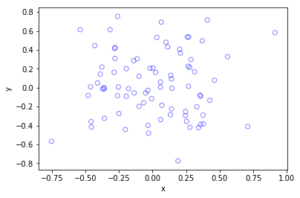
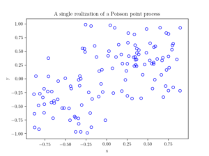
#Plotting a simulation
fig1 = plt.figure();
plt.scatter(xxRetained,yyRetained, edgecolor='b', facecolor='none');
plt.xlabel("x"); plt.ylabel("y");
plt.title('A single realization of a Poisson point process');
plt.show();

#run empirical test on number of points generated
###START -- Checking number of points -- START###
#total mean measure (average number of points)
LambdaNumerical=integrate.dblquad(fun_lambda,xMin,xMax,lambda x: yMin,lambda y: yMax)[0];
#Test: as numbSim increases, numbPointsMean converges to LambdaNumerical
numbPointsMean=np.mean(numbPointsRetained);
#Test: as numbSim increases, numbPointsVar converges to LambdaNumerical
numbPointsVar=np.var(numbPointsRetained);
binEdges=np.arange(numbPointsRetained.min(),(numbPointsRetained.max()+1))-0.5;
pdfEmp, binEdges=np.histogram(numbPointsRetained, bins=binEdges,density=True);

nValues=np.arange(numbPointsRetained.min(),numbPointsRetained.max());
#analytic solution of probability density
pdfExact=(poisson.pmf(nValues,LambdaNumerical));

#Plotting
fig2 = plt.figure();
plt.scatter(nValues,pdfExact, color='b', marker='s',facecolor='none',label='Exact');
plt.scatter(nValues,pdfEmp, color='r', marker='+',label='Empirical');
plt.xlabel("n"); plt.ylabel("P(N=n)");
plt.title('Distribution of the number of points');
plt.legend();
plt.show();
###END -- Checking number of points -- END###

###START -- Checking locations -- START###
#2-D Histogram section
p_Estimate, xxEdges, yyEdges = np.histogram2d(xxAll, yyAll,bins=numbBins,density=True);
lambda_Estimate=p_Estimate*numbPointsMean;

xxValues=(xxEdges[1:]+xxEdges[0:xxEdges.size-1])/2;
yyValues=(yyEdges[1:]+yyEdges[0:yyEdges.size-1])/2;
X, Y = np.meshgrid(xxValues,yyValues) #create x/y matrices for plotting

#analytic solution of probability density
lambda_Exact=fun_lambda(X,Y);

#Plot empirical estimate
fig3 = plt.figure();
plt.rc('text', usetex=True);
plt.rc('font', family='serif');
ax=plt.subplot(211,projection='3d');
surf = ax.plot_surface(X, Y,lambda_Estimate,cmap=plt.cm.plasma);
plt.xlabel("x"); plt.ylabel("y");
plt.title('Estimate of $\lambda(x)$');
plt.locator_params(axis='x', nbins=5);
plt.locator_params(axis='y', nbins=5);
plt.locator_params(axis='z', nbins=3);
#Plot exact expression
ax=plt.subplot(212,projection='3d');
surf = ax.plot_surface(X, Y,lambda_Exact,cmap=plt.cm.plasma);
plt.xlabel("x"); plt.ylabel("y");
plt.title('True $\lambda(x)$');
plt.locator_params(axis='x', nbins=5);
plt.locator_params(axis='y', nbins=5);
plt.locator_params(axis='z', nbins=3);
###END -- Checking locations -- END###

For the histogram section, I used the histogram and histogram2d functions respectively to estimate the distribution of the number of points and the intensity function. I used the pdf option. (The SciPy website recommends not using the the normed option.)

Number of points

np.histogram(numbPointsRetained, bins=binEdges,density=True);

Locations of points

np.histogram2d(xxArrayAll, yyArrayAll,bins=numbBins,density=True);

Simulating an inhomogeneous Poisson point process

In previous posts I described how to simulate homogeneous Poisson point processes on a rectangle, disk and triangle. But here I will simulate an inhomogeneous or nonhomogeneous Poisson point process. (Both of these terms are used, where the latter is probably more popular, but I prefer the former.) For such a point process, the points are not uniformly located on the underlying mathematical space on which the Poisson process is defined. This means that certain regions will, on average, tend to have more (or less) points than other regions of the underlying space.

Basics

Any Poisson point process is defined with a non-negative measure called the intensity or mean measure. I make the standard assumption that the intensity measure \(\Lambda\) has a derivative \(\lambda(x,y)\). (I usually write a single \(x\) to denote a point on the plane, that is \(x\in \mathbb{R}^2\), but in this post I will write the \(x\) and \(y\) and coordinates separately.) The function \(\lambda(x,y)\) is often called the intensity function or just intensity, which I further assume is bounded, so \(\lambda(x,y)<\infty\) for all points in a simulation window \(W\). Finally, I assume that the simulation window \(W\) is a rectangle, but later I describe how to lift that assumption.

Number of points

To simulate a point process, the number of points and the point locations in the simulation window \(W\) are needed. For any Poisson point process, the number of points is a Poisson random variable with a parameter (that is, a mean) \(\Lambda(W)\), which under our previous assumptions is given by the integral

$$\Lambda(W)=\int_W \lambda(x,y)dxdy. $$

Assuming we can evaluate such an integral analytically or numerically, then the number of points is clearly not difficult to simulate.

Locations of points

The difficulty lies in randomly positioning the points. But a defining property of the Poisson point process is its independence, which allows us to treat each point completely independently. Positioning each point then comes down to suitably simulating two (or more) random variables for Poisson point processes in two (or higher) dimensions. Similarly, the standard methods used for simulating continuous random variables can be applied to simulating random point locations of a Poisson point process.

In theory, you can rescale the intensity function with the total measure of the simulation window, giving

$$f(x,y):=\frac{\lambda(x,y)}{\Lambda(W)}. $$

We can then interpret this rescaled intensity function \(f(x,y)\) as the joint probability density of two random variables \(X\) and \(Y\), because it integrates to one,

$$\int_W f(x,y)dxdy=1.$$

Clearly the method for simulating an inhomogeneous Poisson point process depends on the nature of the intensity function. For the inhomogeneous case, the random variables \(X\) and \(Y\) are, in general, not independent.

Transformation

To simulate an inhomogeneous Poisson point process, one method is to first simulate a homogeneous one, and then suitably transform the points according to deterministic function. For simple random variables, this transformation method is quick and easy to implement, if we can invert the probability distribution. For example, a uniform random variable \(U\) defined on the interval \((0,1)\) can be used to give an exponential random variable by applying the transformation \(h(u)= -(1/\lambda)\log(u)\), where \(\lambda>0\), meaning \(h(U)\) is an exponential random variable with parameter \(\lambda>0\) (or mean \(1/\lambda\)).

Similarly for Poisson point processes, the transformation approach is fairly straightforward in a one-dimensional setting, but generally doesn’t work easily in two (or higher) dimensions. The reason being that often we cannot simulate the random variables \(X\) and \(Y\) independently, which means, in practice, we need first to simulate one random variable, then the other.

It is a bit easier if we can re-write the rescaled intensity function or joint probability density \(f(x,y)\) as a product of single-variable functions \(f_X(x)\) and \(f_Y(y)\), meaning the random variables \(X\) and \(Y\) are independent. We can then simulate independently the random variables \(X\) and \(Y\), corresponding to the \(x\) and \(y\) coordinates of the points. But this would still require integrating and inverting the functions.

Markov chain Monte Carlo

A now standard way to simulate jointly distributed random variables is to use Markov chain Monte Carlo (MCMC), which we can also use to simulate the the \(X\) and \(Y\) random variables. Applying MCMC methods is simply applying random point process operations repeatedly to all the points. But this is a bit too tricky and involved. Instead I’ll use a general yet simpler method based on thinning.

Thinning

The thinning method is the arguably the simplest and most general way to simulate an inhomogeneous Poisson point process. If you’re unfamiliar with thinning, I recommend my previous post on thinning and the material I cite.

This simulation method is simply a type of acceptance-rejection method for simulating random variables. More specifically, it is the acceptance-rejection or rejection method, attributed to the great John von Neumann, for simulating a continuous random variable, say \(X\), with some known probability density \(f(x)\). The method accepts/retains or rejects/thins the outcome of each random variable/point depending on the outcome of a uniform random variable associated with each random variable/point.

The thinning or acceptance-rejection method is also appealing because it is an example of a perfect simulation method, which means the distribution of the simulated random variables or points will not be an approximation. This can be contrasted with typical MCMC methods, which, in theory, reach the desired distribution of the random variables in infinite time, which is clearly not possible in practice.

Simulating the homogeneous Poisson point process

First simulate a homogeneous Poisson point process with intensity value \(\lambda^*\), which is an upper bound of the intensity function \(\lambda(x,y)\). The simulation step is the easy part, but what value is \(\lambda^*\)?

I will use the maximum value that the intensity function \(\lambda(x,y)\) takes, which I denote by

$$ \lambda_{\max}:=\max_{(x,y)\in W}\lambda(x,y),$$

so I set \(\lambda^*=\lambda_{\max}\). Of course with \(\lambda^*\) being an upper bound, you can use any larger \(\lambda\)-value, so \(\lambda^*\geq \lambda_{\max}\), but that just means more points will need to be thinned.

Scientific programming languages have implemented algorithms that find or estimate minima of mathematical functions, meaning such an algorithm just needs to find the \((x,y)\) point that gives the minimum value of \(-\lambda(x,y)\), which corresponds to the maximum value of \(\lambda(x,y)\). What is very important is that the minimization procedure can handle constraints on the \(x\) and \(y\) values, which in our case of a rectangular simulation window \(W\) are sometimes called box constraints.

Thinning the Poisson point process

All we need to do now is to thin the homogeneous Poisson point process with the thinning probability function

$$1-p(x,y)=\frac{\lambda(x,y)}{\lambda^*}.$$

This will randomly remove the points so the remaining points will form a inhomogeneous Poisson point process with intensity function
$$ (1-p(x,y))\lambda^* =\lambda(x,y).$$
As a result, we can see that provided \(\lambda^*\geq \lambda_{\max}>0\), this procedure will give the right intensity function \(\lambda(x,y)\). I’ll skip the details on the point process still being Poisson after thinning, as I have already covered this in the thinning post.

Empirical check

You can run an empirical check by simulating the point process a large number (say \(10^3\) or \(10^4\)) of times, and collect statistics on the number of points. As the number of simulations increases, the average number of points should converge to the intensity measure \(\Lambda(W)\), which is given by (perhaps numerically) evaluating the integral

$$\Lambda(W)=\int_W \lambda(x,y)dxdy.$$

This is a test for the intensity measure, a type of first moment, which will work for the intensity measure of any point process. But for Poisson point processes, the variance of the number of points will also converge to intensity measure \(\Lambda(W)\), giving a second empirical test based on second moments.

An even more thorough test would be estimating an empirical distribution (that is, performing and normalizing a histogram) on the number of points. These checks will validate the number of points, but not the positioning of the points. In my next post I’ll cover how to perform these tests.

Results

The homogeneous Poisson point process with intensity function \(\lambda(x)=100\exp(-(x^2+y^2)/s^2)\), where \(s=0.5\). The results look similar to those in the thinning post, where the thinned points (that is, red circles) are generated from the same Poisson point process as the one that I have presented here.

MATLAB

Python

Method extensions

We can extend the thinning method for simulating inhomogeneous Poisson point processes a couple different ways.

Using an inhomogeneous Poisson point process

The thinning method does not need to be applied to a homogeneous Poisson point process with intensity \(\lambda^*\). In theory, we could have simulated a suitably inhomogeneous Poisson point process with intensity function \(\lambda^*(x,y)\), which has the condition

$$ \lambda^*(x,y)\geq \lambda(x,y), \quad \forall (x,y)\in W .$$

Then this Poisson point process is thinned. But then we would still need to simulate the underlying Poisson point process, which often would be as difficult to simulate.

Partitioning the simulation window

Perhaps the intensity of the Poisson point process only takes two values, \(\lambda_1\) and \(\lambda_2\), and the simulation window \(W\) can be nicely divided or partitioned into two disjoints sets \(B_1\) and \(B_2\) (that is, \(B_1\cap B_2=\emptyset\) and \(B_1\cup B_2=W\)), corresponding to the subregions of the two different intensity values. The Poisson independence property allows us to simulate two independent Poisson point processes on the two subregions.

This approach only works for a piecewise constant intensity function. But if if the intensity function \(\lambda(x)\) varies wildly, the simulation window can be partitioned into subregions \(B_1\dots,B_m\) for different ranges of the intensity function \(\lambda(x)\). This allows us to simulate independent homogeneous Poisson point processes with different densities \(\lambda^*_1\dots, \lambda^*_m\), where for each subregion \(B_i\) we set

$$ \lambda^*_i:=\max_{x\in B_i}\lambda(x,y).$$

The resulting Poisson point processes are then suitably thinned, resulting in a more efficient simulation method. (Although I imagine the gain would often be small.)

Non-rectangular simulation windows

If you want to simulate on non-rectangular regions, which is not a disk or triangle, then the easiest way is to simulate a Poisson point process on a rectangle \(R\) that completely covers the simulation window, so \(W \subset R\subset \mathbb{R}^2\), and then set the intensity function \(\lambda \) to zero for the region outside the simulation window \(W\), that is \(\lambda (x,y)=0\) when \((x,y)\in R\setminus W\).

Further reading

In Section 2.5.2 of Stochastic Geometry and its Applications by Chiu, Stoyan, Kendall and Mecke, there is an outline of the thinning method that I used. The same simulation section appears in the previous edition by Kendall and Mecke, though these books in general have little material on simulation methods.

More details on the thinning method and its connection to acceptance-rejection sampling are given in Section 2.3 of the applications-oriented book Poisson Point Processes by Streit. The acceptance-rejection method is covered in, for example, books on Monte Carlo methods, including Monte Carlo Strategies in Scientific Computing by Liu (in Section 2.2 )and Monte Carlo Methods in Financial Engineering by Glasserman (in Section 2.2.2). This method and others for simulating generals random variable are covered in stochastic simulation books such as Uniform Random Variate Generation by Devroye and Stochastic Simulation: Algorithms and Analysis by Asmussen and Glynn.

Kroese and Botev have a good introduction to stochastic simulation in the edited collection Stochastic Geometry, Spatial Statistics and Random Fields : Models and Algorithms by Schmidt, where the relevant chapter (number 12) is also freely available online. And of course there are lectures notes on the internet that cover simulation material.

Code

All code from my posts, as always, can be found on the my GitHub repository. The code for this post is located here. You can see that the code is very similar to that of the thinning code, which served as the foundation for this code. (Note how we now keep the points, so in the code the > has become < on the line where the uniform variables are generated).

I have implemented the code in MATLAB and Python with an intensity function \(\lambda(x,y)=100\exp(-(x^2+y^2)/s^2)\), where \(s>0\) is a scale parameter. Note that in the minimization step, the box constraints are expressed differently in MATLAB and Python: MATLAB first takes the minimum values then the maximum values, whereas Python first takes the \(x\)-values then the \(y\)-values.

The code presented here does not have the empirical check, which I described above, but it is implemented in the code located here. For the parameters used in the code, the total measure is \(\Lambda(W)\approx 77.8068\), meaning each simulation will generate on average almost seventy-eight points.

I have stopped writing code in R for a couple of reasons, but mostly because anything I could think of simulating in R can already be done in the spatial statistics library spatstat. I recommend the book Spatial Point Patterns, co-authored by the spatstat’s main contributor, Adrian Baddeley.

MATLAB

I have used the fmincon function to find the point that gives the minimum of \(-\lambda(x,y)\).

%Simulation window parameters
xMin=-1;xMax=1;
yMin=-1;yMax=1;
xDelta=xMax-xMin;yDelta=yMax-yMin; %rectangle dimensions
areaTotal=xDelta*yDelta; %area of rectangle

s=0.5; %scale parameter

%Point process parameters
fun_lambda=@(x,y)(100*exp(-((x).^2+(y).^2)/s^2));%intensity function

%%%START -- find maximum lambda -- START %%%
%For an intensity function lambda, given by function fun_lambda,
%finds the maximum of lambda in a rectangular region given by
%[xMin,xMax,yMin,yMax].
funNeg=@(x)(-fun_lambda(x(1),x(2))); %negative of lambda
%initial value(ie centre)
xy0=[(xMin+xMax)/2,(yMin+yMax)/2];%initial value(ie centre)
%Set up optimization step
options=optimoptions('fmincon','Display','off');
%Find largest lambda value
[~,lambdaNegMin]=fmincon(funNeg,xy0,[],[],[],[],...
[xMin,yMin],[xMax,yMax],'',options);
lambdaMax=-lambdaNegMin;
%%%END -- find maximum lambda -- END%%%

%define thinning probability function
fun_p=@(x,y)(fun_lambda(x,y)/lambdaMax);

%Simulate Poisson point process
numbPoints=poissrnd(areaTotal*lambdaMax);%Poisson number of points
xx=xDelta*(rand(numbPoints,1))+xMin;%x coordinates of Poisson points
yy=xDelta*(rand(numbPoints,1))+yMin;%y coordinates of Poisson points

%calculate spatially-dependent thinning probabilities
p=fun_p(xx,yy);

%Generate Bernoulli variables (ie coin flips) for thinning
booleRetained=rand(numbPoints,1)<p; %points to be thinned

%x/y locations of retained points
xxRetained=xx(booleRetained); yyRetained=yy(booleRetained);

%Plotting
plot(xxRetained,yyRetained,'bo'); %plot retained points
xlabel('x');ylabel('y');

The box constraints for the optimization step were expressed as:

[xMin,yMin],[xMax,yMax]
Python

I have used the minimize function in SciPy.

import numpy as np; #NumPy package for arrays, random number generation, etc
import matplotlib.pyplot as plt #For plotting
from scipy.optimize import minimize #For optimizing
from scipy import integrate

#Simulation window parameters
xMin=-1;xMax=1;
yMin=-1;yMax=1;
xDelta=xMax-xMin;yDelta=yMax-yMin; #rectangle dimensions
areaTotal=xDelta*yDelta;

s=0.5; #scale parameter

#Point process parameters
def fun_lambda(x,y):
return 100*np.exp(-(x**2+y**2)/s**2); #intensity function

###START -- find maximum lambda -- START ###
#For an intensity function lambda, given by function fun_lambda,
#finds the maximum of lambda in a rectangular region given by
#[xMin,xMax,yMin,yMax].
def fun_Neg(x):
return -fun_lambda(x[0],x[1]); #negative of lambda

xy0=[(xMin+xMax)/2,(yMin+yMax)/2];#initial value(ie centre)
#Find largest lambda value
resultsOpt=minimize(fun_Neg,xy0,bounds=((xMin, xMax), (yMin, yMax)));
lambdaNegMin=resultsOpt.fun; #retrieve minimum value found by minimize
lambdaMax=-lambdaNegMin;
###END -- find maximum lambda -- END ###

#define thinning probability function
def fun_p(x,y):
return fun_lambda(x,y)/lambdaMax;

#Simulate a Poisson point process
numbPoints = np.random.poisson(lambdaMax*areaTotal);#Poisson number of points
xx = np.random.uniform(0,xDelta,((numbPoints,1)))+xMin;#x coordinates of Poisson points
yy = np.random.uniform(0,yDelta,((numbPoints,1)))+yMin;#y coordinates of Poisson points

#calculate spatially-dependent thinning probabilities
p=fun_p(xx,yy);

#Generate Bernoulli variables (ie coin flips) for thinning
booleRetained=np.random.uniform(0,1,((numbPoints,1)))<p; #points to be thinned

#x/y locations of retained points
xxRetained=xx[booleRetained]; yyRetained=yy[booleRetained];

#Plotting
plt.scatter(xxRetained,yyRetained, edgecolor='b', facecolor='none', alpha=0.5 );
plt.xlabel("x"); plt.ylabel("y");
plt.show();

The box constraints were expressed as:

(xMin, xMax), (yMin, yMax)
Julia

After writing this post, I later wrote the code in Julia. The code is here and my thoughts about Julia are here.

Thinning point processes

One way to create new point processes is to apply thinning to a point process. As I mentioned in a previous post on point process operations, thinning is a random operation applied to the points of an underlying point process, where the points are thinned (or removed) or retained (or kept) according to some probabilistic rule. Both the thinned and retained points form two separate point processes, but one usually focuses on the retained points. Given an underlying point process, the nature of the thinning rule will result in different types of point processes.

As I detailed in the Applications section below, thinning can be used to simulate an inhomogeneous Poisson point process, as I covered in another post.

Thinning types

Thinning can be statistically independent or dependent, meaning that the probability of thinning any point is either independent or dependent of thinning other points. The more tractable case is statistically independent thinning, which is the thinning type covered here. We can further group this thinning into two types based on whether the thinning rule depends on the locations of the point. (I use the word location, instead of point, to refer to where a point of a point process is located on the underlying mathematical space on which the point process is defined.)

Spatially independent thinning

The simplest thinning operation is one that does not depend on point locations. This thinning is sometimes referred to as \(p\)-thinning, where the constant \(p\) has the condition \(0\leq p \leq 1\) because it is the probability of thinning a single point. Simply put, the probability of a point being thinned does not depend on the point locations.

Example

We can liken the thinning action to flipping a biased coin with probability of \(p\) for heads (or tails) for each point of the underlying point process, and then removing the point if a head (or tails) occurs. If there were a constant number \(n\) of points of the underlying point process, then the number of thinned (or retained) points will form a binomial random variable with parameters \(n\) and \(p\) (or \(1-p\)).

Simulation

Simulating this thinning operation is rather straightforward. Given a realization of a point process, for each point, simply generate or simulate a uniform random variable on the interval \((0,1)\), and if this random variable is less than \(p\), remove the point. (This is simply sampling a Bernoulli distribution, which is covered in this post.)

In the code section below, I have shown how this thinning operation is implemented.

Spatially dependent thinning

To generalize the idea of \(p\)-thinning, we can simply require that the thinning probability of any point depends on its location \(x\), which gives us the concept of \(p(x)\)-thinning. (I write a single \(x\) to denote a point on the plane, that is \(x\in \mathbb{R}^2\), instead of writing, for example, the \(x\) and \(y\) and coordinates separately.) More precisely, the probability of thinning a point is given by a function \(p(x)\) such that \(0 \leq p(x)\leq 1\), but all point thinnings occur independently of each other. In other words, this is a spatially dependent thinning that is statistically independent.

Example

I’ll illustrate the concept of (statistically independent) spatially dependent thinning with a somewhat contrived example. We assume that the living locations of all the people in the world form a point process on a (slightly squashed) sphere. Let’s say that Earth has become overpopulated, particularly in the Northern Hemisphere, so we decide to randomly choose people and send them off to another galaxy, but we do it based on how far they live from the North Pole. The thinning rule could be, for example, \(p(x)= \exp(- |x|^2/s^2)\), where \(|x|\) is the distance to the North Pole and \(s>0\) is some constant for distance scaling.

Put another way, a person at location \(x\) flips a biased coin with the probability of heads being equal to \(p(x)=\exp(- |x|^2/s^2)\). If a head comes up, then that person is removed from the planet. With the maximum of \(p(x)\) is at the North Pole, we can see that the lucky (or unlucky?) people in countries like Australia, New Zealand (or Aotearoa), South Africa, Argentina and Chile, are more likely not to be sent off (that is, thinned) into the great unknown.

For people who live comparable distances from the North Pole, the removal probabilities are similar in value, yet the events of being remove remain independent. For example, the probabilities of removing any two people from the small nation Lesotho are similar in value, but these two random events are still completely independent of each other.

Simulation

Simulating a spatially dependent thinning is just slightly more involved than the spatially independent case. Given a realization of a point process, for each point at, say, \(x\), simply generate or simulate a uniform random variable on the interval \((0,1)\), and if this random variable is less than \(p(x)\), remove the point.

In the code section, I have shown how this thinning operation is implemented with an example like the above one, but on a rectangular region of Cartesian space. In this setting, the maximum of \(p(x)\) is at the origin, resulting in more points being thinned in this region.

Thinning a Poisson point process

Perhaps not surprisingly, under the thinning operation the Poisson point process exhibits a closure property, meaning that a Poisson point process thinned in a certain way gives another Poisson point process.  More precisely, if the thinning operation is statistically independent, then the resulting point process formed from the retained points is also a Poisson point process, regardless if it is spatially independent or dependent thinning. The resulting intensity (interpreted as the average density of points) of this new Poisson point process has a simple expression.

Homogeneous case

For a spatially independent \(p\)-thinning, if the original (or underlying) Poisson point process is homogeneous with intensity \(\lambda\), then the point process formed from the retained points is a homogeneous Poisson point process with intensity \(\lambda\).  (There are different ways to prove this, but you can gain some intuition behind the proof by conditioning on the Poisson number of points and then applying the total law of probability. Using generating functions helps.)

Inhomogeneous case

More generally, if we apply a spatially dependent \(p(x)\)-thinning to a  Poisson point process has a intensity \(\lambda\), then the retained points form a  an inhomogeneous or nonhomogeneous Poisson point process with \(\lambda p(x)\),  due to the spatial dependence in the thinning function \(p(x)\). This gives a way to simulate such Poisson point processes, which I’ll cover in another post.

Splitting

We can see by symmetry that if we look at the thinned points, then the resulting point process is also a Poisson point process, but with intensity \((1-p(x))\lambda\). The retained and thinned points both form Poisson point processes, but what is really interesting is these two point processes are independent of each other.  This means that any random configuration that occurs among the retained points is independent of any configurations among the thinned points.

This ability to split a Poisson point processes into independent ones is sometimes called the splitting property.

Applications

Thinning point processes has the immediate application of creating new point processes. It can also be used to randomly generate two point processes from one. In network applications, a simple example is using the thinning procedure to model random sleep schemes in wireless networks, where random subsets of the network have been powered down.

Perhaps the most useful application of thinning is creating point processes with spatially-dependent intensities such that of an inhomogeneous Poisson point process. In another post I give details on how to simulate this point process.  In this setting, the thinning operation essentially is acceptance(-rejection) sampling, which I will cover in a future post.

Code

All code from my posts, as always, can be found on the my GitHub repository. The code for this post is located here.

Spatially independent thinning

I have implemented in code the simple \(p\)-thinning operation applied to a Poisson point process on a rectangle, but in theory any point process can be used for the underlying point process that is thinned.

MATLAB

%Simulation window parameters
xMin=-1;xMax=1;
yMin=-1;yMax=1;
xDelta=xMax-xMin;yDelta=yMax-yMin; %rectangle dimensions
areaTotal=xDelta*yDelta; %area of rectangle

%Point process parameters
lambda=100; %intensity (ie mean density) of the Poisson process

%Thinning probability parameters
sigma=1;
p=0.25; %thinning probability

%Simulate Poisson point process
numbPoints=poissrnd(areaTotal*lambda);%Poisson number of points
xx=xDelta*(rand(numbPoints,1))+xMin;%x coordinates of Poisson points
yy=xDelta*(rand(numbPoints,1))+yMin;%y coordinates of Poisson points

%Generate Bernoulli variables (ie coin flips) for thinning
booleThinned=rand(numbPoints,1)&amp;amp;gt;p; %points to be thinned
booleRetained=~booleThinned; %points to be retained

%x/y locations of thinned points
xxThinned=xx(booleThinned); yyThinned=yy(booleThinned);
%x/y locations of retained points
xxRetained=xx(booleRetained); yyRetained=yy(booleRetained);

%Plotting
plot(xxRetained,yyRetained,'bo'); %plot retained points
hold on; plot(xxThinned,yyThinned,'ro'); %plot thinned points
xlabel('x');ylabel('y');

R

#Simulation window parameters
xMin=-1;xMax=1;
yMin=-1;yMax=1;
xDelta=xMax-xMin;yDelta=yMax-yMin; #rectangle dimensions
areaTotal=xDelta*yDelta;

#Point process parameters
lambda=100; #intensity (ie mean density) of the Poisson process

#Thinning probability
p=0.25; 

#Simulate a Poisson point process
numbPoints=rpois(1,areaTotal*lambda);#Poisson number of points
xx=xDelta*runif(numbPoints)+xMin;#x coordinates of Poisson points
yy=xDelta*runif(numbPoints)+yMin;#y coordinates of Poisson points

#Generate Bernoulli variables (ie coin flips) for thinning
booleThinned=runif(numbPoints)&amp;amp;gt;p; #points to be thinned
booleRetained=!booleThinned; #points to be retained

#x/y locations of thinned points
xxThinned=xx[booleThinned]; yyThinned=yy[booleThinned];
#x/y locations of retained points
xxRetained=xx[booleRetained]; yyRetained=yy[booleRetained];

#Plotting
par(pty="s")
plot(xxRetained,yyRetained,'p',xlab='x',ylab='y',col='blue'); #plot retained points
points(xxThinned,yyThinned,col='red'); #plot thinned points

Of course, as I have mentioned before, simulating a spatial point processes in R is even easier with the powerful spatial statistics library spatstat.  With this library, thinning can be done in quite a general way by using the function rthin.

Python

import numpy as np; #NumPy package for arrays, random number generation, etc
import matplotlib.pyplot as plt

#Simulation window parameters
xMin=-1;xMax=1;
yMin=-1;yMax=1;
xDelta=xMax-xMin;yDelta=yMax-yMin; #rectangle dimensions
areaTotal=xDelta*yDelta;

#Point process parameters
lambda0=100; #intensity (ie mean density) of the Poisson process

#Thinning probability
p=0.25; 

#Simulate a Poisson point process
numbPoints = np.random.poisson(lambda0*areaTotal);#Poisson number of points
xx = np.random.uniform(0,xDelta,((numbPoints,1)))+xMin;#x coordinates of Poisson points
yy = np.random.uniform(0,yDelta,((numbPoints,1)))+yMin;#y coordinates of Poisson points

#Generate Bernoulli variables (ie coin flips) for thinning
booleThinned=np.random.uniform(0,1,((numbPoints,1)))&amp;amp;gt;p; #points to be thinned
booleRetained=~booleThinned; #points to be retained

#x/y locations of thinned points
xxThinned=xx[booleThinned]; yyThinned=yy[booleThinned];
#x/y locations of retained points
xxRetained=xx[booleRetained]; yyRetained=yy[booleRetained];

#Plotting
plt.scatter(xxRetained,yyRetained, edgecolor='b', facecolor='none', alpha=0.5 );
plt.scatter(xxThinned,yyThinned, edgecolor='r', facecolor='none', alpha=0.5 );
plt.xlabel("x"); plt.ylabel("y");
plt.show(); 
Spatially dependent thinning

I have implemented in code a \(p(x)\)-thinning operation with the function \(p(x)=\exp(-|x|^2/s^2)\), where \(|x|\) is the Euclidean distance from \(x\) to the origin. This small changes means that in the code there will be a vector or array of \(p\) values instead of a single \(p\) value in the section where the uniform random variables are generated and compared said \(p\) values.  (Lines 24, 26 and 28 respectively in the MATLAB, R and Python code presented below.)

Again, I have applied thinning to a Poisson point process on a rectangle, but in theory any point process can be used for the underlying point process.

MATLAB

%Simulation window parameters
xMin=-1;xMax=1;
yMin=-1;yMax=1;
xDelta=xMax-xMin;yDelta=yMax-yMin; %rectangle dimensions
areaTotal=xDelta*yDelta; %area of rectangle
 
%Point process parameters
lambda=100; %intensity (ie mean density) of the Poisson process

%Thinning probability parameters
sigma=0.5; %scale parameter for thinning probability function
%define thinning probability function
fun_p=@(s,x,y)(exp(-(x.^2+y.^2)/s^2)); 

%Simulate Poisson point process
numbPoints=poissrnd(areaTotal*lambda);%Poisson number of points
xx=xDelta*(rand(numbPoints,1))+xMin;%x coordinates of Poisson points
yy=xDelta*(rand(numbPoints,1))+yMin;%y coordinates of Poisson points

%calculate spatially-dependent thinning probabilities
p=fun_p(sigma,xx,yy); 

%Generate Bernoulli variables (ie coin flips) for thinning
booleThinned=rand(numbPoints,1)&amp;amp;gt;p; %points to be thinned
booleRetained=~booleThinned; %points to be retained

%x/y locations of thinned points
xxThinned=xx(booleThinned); yyThinned=yy(booleThinned);
%x/y locations of retained points
xxRetained=xx(booleRetained); yyRetained=yy(booleRetained);

%Plotting
plot(xxRetained,yyRetained,'bo'); %plot retained points
hold on; plot(xxThinned,yyThinned,'ro'); %plot thinned points
xlabel('x');ylabel('y');

R

#Simulation window parameters
xMin=-1;xMax=1;
yMin=-1;yMax=1;
xDelta=xMax-xMin;yDelta=yMax-yMin; #rectangle dimensions
areaTotal=xDelta*yDelta;

#Point process parameters
lambda=100; #intensity (ie mean density) of the Poisson process

#Thinning probability parameters
sigma=0.5; #scale parameter for thinning probability function
#define thinning probability function
fun_p &amp;amp;lt;- function(s,x,y) {
  exp(-(x^2 + y^2)/s^2);
}

#Simulate a Poisson point process
numbPoints=rpois(1,areaTotal*lambda);#Poisson number of points
xx=xDelta*runif(numbPoints)+xMin;#x coordinates of Poisson points
yy=xDelta*runif(numbPoints)+yMin;#y coordinates of Poisson points

#calculate spatially-dependent thinning probabilities
p=fun_p(sigma,xx,yy); 

#Generate Bernoulli variables (ie coin flips) for thinning
booleThinned=runif(numbPoints)&amp;amp;lt;p; #points to be thinned
booleRetained=!booleThinned; #points to be retained

#x/y locations of thinned points
xxThinned=xx[booleThinned]; yyThinned=yy[booleThinned];
#x/y locations of retained points
xxRetained=xx[booleRetained]; yyRetained=yy[booleRetained];

#Plotting
par(pty="s")
plot(xxRetained,yyRetained,'p',xlab='x',ylab='y',col='blue'); #plot retained points
points(xxThinned,yyThinned,col='red'); #plot thinned points

Again, use the spatial statistics library spatstat, which has the function rthin.

Python

import numpy as np; #NumPy package for arrays, random number generation, etc
import matplotlib.pyplot as plt

#Simulation window parameters
xMin=-1;xMax=1;
yMin=-1;yMax=1;
xDelta=xMax-xMin;yDelta=yMax-yMin; #rectangle dimensions
areaTotal=xDelta*yDelta;

#Point process parameters
lambda0=100; #intensity (ie mean density) of the Poisson process

#Thinning probability parameters
sigma=0.5; #scale parameter for thinning probability function
#define thinning probability function
def fun_p(s, x, y):
    return np.exp(-(x**2+y**2)/s**2);    

#Simulate a Poisson point process
numbPoints = np.random.poisson(lambda0*areaTotal);#Poisson number of points
xx = np.random.uniform(0,xDelta,((numbPoints,1)))+xMin;#x coordinates of Poisson points
yy = np.random.uniform(0,yDelta,((numbPoints,1)))+yMin;#y coordinates of Poisson points

#calculate spatially-dependent thinning probabilities
p=fun_p(sigma,xx,yy); 

#Generate Bernoulli variables (ie coin flips) for thinning
booleThinned=np.random.uniform(0,1,((numbPoints,1)))&amp;amp;gt;p; #points to be thinned
booleRetained=~booleThinned; #points to be retained

#x/y locations of thinned points
xxThinned=xx[booleThinned]; yyThinned=yy[booleThinned];
#x/y locations of retained points
xxRetained=xx[booleRetained]; yyRetained=yy[booleRetained];

#Plotting
plt.scatter(xxRetained,yyRetained, edgecolor='b', facecolor='none', alpha=0.5 );
plt.scatter(xxThinned,yyThinned, edgecolor='r', facecolor='none', alpha=0.5 );
plt.xlabel("x"); plt.ylabel("y");
plt.show(); 

Results

In the plotted results, the blue and red circles represent respectively the retained and thinned points.

Spatially independent thinning

For these results, I used a thinning probability \(p=0.25\), which means that roughly a quarter of the points will be thinned, so on average the ratio of blue to red circles is three to one.

MATLAB

R

Python

Spatially dependent thinning

Observe how there are more thinned points (that is, red circles) near the origin, which is of course where the thinning function \(p(x)=\exp(-|x|^2/s^2)\) attains its maximum.

MATLAB

R

Python

Further reading

The thinning operation is covered in Stochastic Geometry and its Applications by Chiu, Stoyan, Kendall and Mecke (Chapter 5). It is also covered in the book Statistical Inference and Simulation for Spatial Point Processes by Moller and Waagepetersen (Section 3.2.2). Kallenberg presents a more theoretical and rigorous take on thinning Poisson point processes in his new book Random Measures, Theory and Applications (Chapter 3). (A point process can be interpreted as a type of random measure called a random counting measure because it gives the random number of points in a set.)

Thinning is also covered in books that apply point processes to wireless networks, such as Stochastic Geometry and Wireless Networks by Baccelli and Błaszczyszyn (Volume 1, Section 1.3.2) or Stochastic Geometry for Wireless Networks (Section 2.7.3) by Haenggi. These books also give examples of thinning point processes for wireless network applications.