Spatial point process Archives

Voronoi tessellations

Cholera outbreaks due to public water pumps. Suburbs serviced by hospitals. Formation of crystals. Coverage regions of phone towers. We can model or approximate all these phenomena and many, many more with a geometric structure called, among other names, a Voronoi tessellation.

The main other name for this object is the Dirichlet tessellation. Historically, Dirichlet beats Voronoi, but it seems wherever I look, the name Voronoi usually wins out, suggesting an example of Stigler’s law of eponymy. A notable exception is the R library spatstat that does actually call it a Dirichlet tessellation. Wikipedia calls it a Voronoi diagram. I’ve read that Descartes studied the object even earlier than Dirichlet, but Voronoi studied it in much more depth. At any rate, I will call it a Voronoi tessellation.

To form a Voronoi tessellation, consider a collection of points scattered on some space, like the plane, where it’s easier to picture things, especially when using a Euclidean metric. Now for each point in the collection, consider the surrounding region that is closer to that point than any other point in the collection. Each region forms a cell corresponding to the point. The union of all the sets covers the underlying space. That union of sets is the Voronoi tessellation.

The evolution of Voronoi cells, which start off as disks until they collide with each other. Source: Wikipedia.

Mathematicians have extensively studied Voronoi tessellations, particularly those based on Poisson point processes, forming a core subject in the field of stochastic geometry.

Everyday Voronoi tessellations

Voronoi tessellations are just not interesting mathematical objects, as they arise in everyday situations. This piece from Scientific American website explains:

Everyone uses Voronoi tessellations, even without realizing it. Individuals seeking the nearest café, urban planners determining service area for hospitals, and regional planners outlining school districts all consider Voronoi tessellations. Each café, school, or hospital is a site from which a Voronoi tessellation is generated. The cells represent ideal service areas for individual businesses, schools, or hospitals to minimize clientele transit time. Coffee drinkers, patients, or students inside a service area (that is, a cell) should live closer to their own café, hospital, or school (that is, their own cell’s site) than any other. Voronoi tessellations are ubiquitous, yet often invisible.

Delaunay triangulation

A closely related object is the Delaunay triangulation. For a given collection of points on some underlying mathematical space, a Delaunay triangulation is formed by connecting the points and creating triangles with the condition that for each point, no other point exists in the circumcircle of the corresponding triangle. (A circumcircle is a circle that passes through all three vertices of a triangle.)

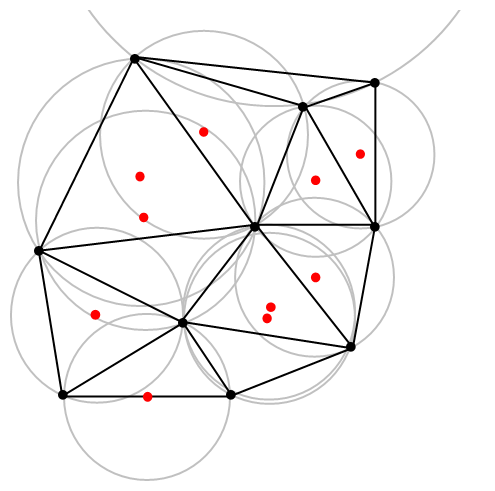
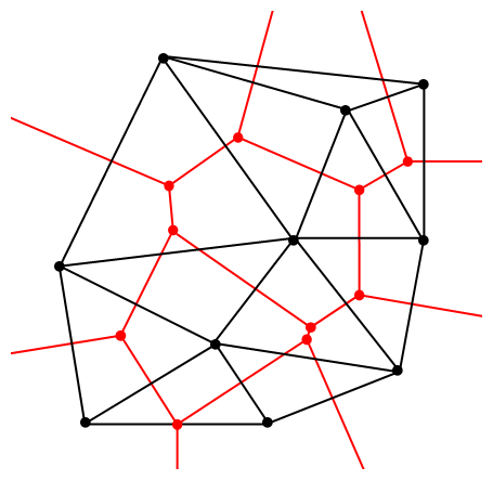
The vertices of the the Delaunay triangular and Voronoi tessellation both form graphs, which turn out to be the dual graphs of each other.

A Delaunay triangulation (in black) and the corresponding Voronoi tessellation (in red) whose vertices are the centres of the circumcircles of the Delaunay triangles. Source: Wikipedia.

Software: Qhull

Due to its applications, it’s not surprising that there exist algorithms that quickly create or estimate Voronoi tessellations. I don’t want to implement one of these algorithms from scratch, as they have already been implemented in various scientific programming languages. Many of the languages, such as MATLAB, R, and Python (SciPy) use the code from Qhull. (Note the Qhull website calls the tessellation a Voronoi diagram.)

(The Julia programming language, which I examined in a previous post, has a Voronoi package that does not use Qhull.)

Qhull finds the Voronoi tessellation by first finding the Delaunay triangulation. If the underlying space is bounded, then all the Voronoi cells are also bounded. But on an unbounded space, it is possible to have unbounded cells, meaning their areas (or volumes) are infinite. In such cases, the algorithms sometime place virtual points at infinity, but I don’t want to focus on such details. I will assume Qhull does a good job.

Code

As always, the code from all my posts is online. For this post, the MATLAB and Python code is here and here, respectively, which generates Voronoi tesselations.

MATLAB

It is fairly straightforward to create Voronoi tessellations in MATLAB. You can just use the function voronoi, which is only for two-dimensional tessellations. (Note: the MATLAB website says the behaviour of the function voronoi has changed, so that may cause problems when using different versions of MATLAB.) The function requires two inputs as vectors, say, x and y, corresponding to the Cartesian (or $x$ and $y$) coordinates of the points. If you just run the voronoi command, it will create and plot a Voronoi tessellation (or Voronoi diagram, as MATLAB calls it). But the MATLAB website also describes how to plot the tessellation manually.

For $d$ -dimensional tessellations, there is the function voronoin, which requires a single input. The single output consists of combining $d$ column vectors for the Cartesian coordinates. For example, given the column vectors x, y and z, then the input is [x, y, z].

If you give the functions voronoi or voronoin output arguments, then the tessellation is not plotted and instead two data structures, say, v and c are created for describing the vertices of the tessellation. I generally use voronoi for plotting, but I use voronoin (and not voronoi) for generating vertex data, so I will focus on the outputs of voronoin.

For voronoin, the first (output) data structure v is simply an two-dimensional array array that contain the Cartesian coordinates of every vertex in the Voronoi tessellation. The second (output) data structure c is a cell array describing the vertices of each Voronoi cell (it has to be a cell array, as opposed to a regular array, as the cells have varying number of vertices). Each entry of the cell array contains a one-dimensional array with array indices corresponding to the $x$ and $y$ coordinates.

The code checks which Voronoi cells are unbounded by seeing if they have vertices at infinity, which corresponds to a $1$ in the index arrays (stored in the structure array c).

One criticism of the MATLAB functions is that they don’t return all the information of the Voronoi tessellation. More specifically, the functions don’t return the boundaries between the unbounded cells, though voronoi internally calculates and uses these boundaries to generate Voronoi plots. This is covered in this review on different Voronoi packages. Conversely, the Python package returns more information such as that of the edges or ridges of the Voronoi cells.

Python

To create the Voronoi tessellation, use the SciPy (Spatial) function Voronoi. This function does $d$-dimensional tessellations. For the two-dimensional setting, you need to input the $x$ and $y$ coordinates as a single array of dimensions $2 \times n$, where $n$ is the number of points in the collection. In my code, I start off with two one-dimensional arrays for the Cartesian coordinates, but then I combined them into a single array by using the function numpy.stack with the function argument axis =1.

I would argue that the Voronoi function in SciPy is not as intuitive to use as the MATLAB version. One thing I found a bit tricky, at first, is that the cells and the points have a different sets of numbering (that is, they are indexed differently). (And I am not the only one that was caught by this.) You must use the attribute called point_region to access a cell number (or index) from a point number (or index). In my code the attribute is accessed and then called it indexP2C, which is an integer array with cell indices. Of course, there could be a reason for this, and I am just failing to understand it.

Apart from the above criticism, the function Voronoi worked well. As I mentioned before, this package returns more Voronoi information than the MATLAB equivalents.

To plot the Voronoi tessellation, use the SciPy function voronoi_plot_2d, which allows for various plotting options, but it does require Matplotlib. The input is the data object created by the function Voronoi.

Results

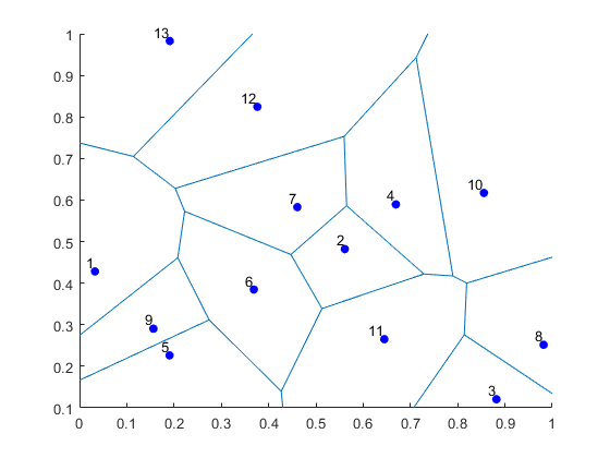
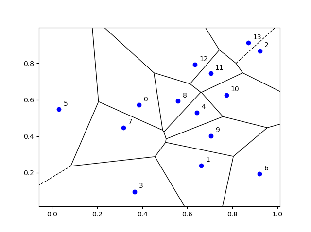
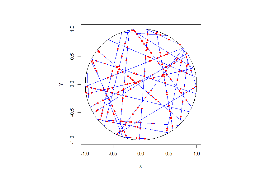
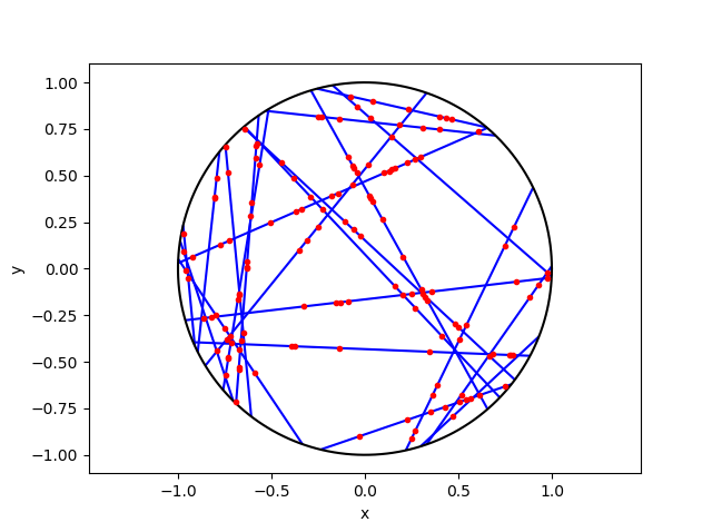
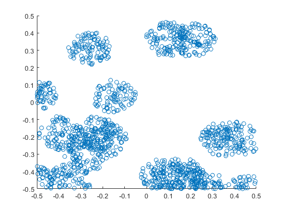
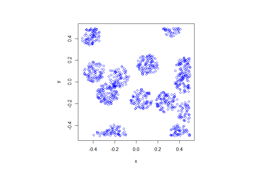
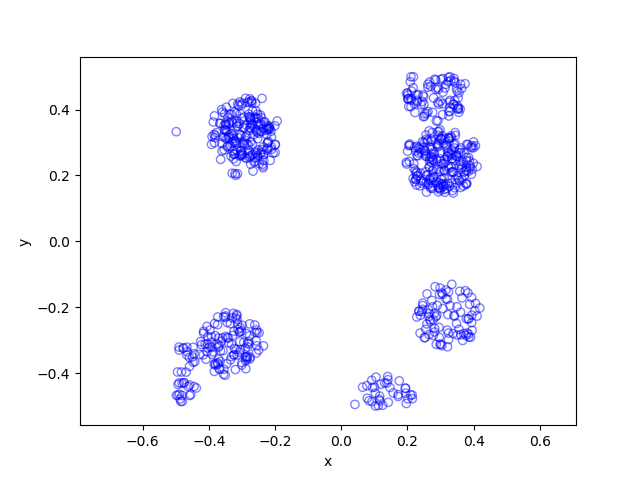
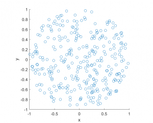
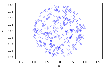
I’ve plotted the results for a single realization of a Poisson point process. I’ve also plotted the indices of the points. Recall that the indexing in Python and MATLAB start respectively at zero and one.

MATLAB

Python

Voronoi animations

I took the animation of evolving Voronoi cells, which appears in the introduction, from Wikipedia. The creator generated it in MATLAB and also posted the code online. The code is long, and I wouldn’t even dare to try to reproduce it, but I am glad someone else wrote it.

Such animations exist also for other metrics. For example, the Manhattan metric (or taxi cab or city block metric) gives the animation below, where the growing disks have been replaced with squares.

A Voronoi tessellation under the Manhattan metric. The evolving cells start off as squares until they collide with each other. Source: Wikipedia.

This Wikipedia user page has animations under other metrics on Euclidean space.

This post also features animations of Voronoi tessellations when the points move.

Simulating a Cox point process based on a Poisson line process

In the previous post, I described how to simulate a Poisson line process, which in turn was done by using insight from an earlier post on the Bertrand paradox.

Now, given a Poisson line process, for each line, if we generate an independent one-dimensional Poisson point point process on each line, then we obtain an example of a Cox point process. Cox point processes are also known as doubly stochastic Poisson point processes. On the topic of names, Guttorp and Thorarinsdottir argue that it should be called the Quenouille point process, as Maurice Quenouille introduced an example of it before Sir David Cox, but I opt for the more common name.

Cox point proceesses

A Cox point process is a generalization of a Poisson point process. It is created by first considering a non-negative random measure, sometimes called a driving measure. Then a Poisson point process, which is independent of the random driving measure, is generated by using the random measure as its intensity or mean measure.

The driving measure of a Cox point process can be, for example, a non-negative random variable or field multiplied by a Lebesgue measure. In our case, the random measure is the underlying Poisson line process coupled with the Lebesgue measure on the line (that is, length).

Cox processes form a very large and general family of point processes, which exhibit clustering. In previous posts, I have covered two special cases of Cox point processes: the Matérn and Thomas cluster point processes. These are, more specifically, examples of a Neyman-Scott point process, which is a special case of a shot noise Cox point process. These two point processes are fairly easy to simulate, but that’s not the case for Cox point processes in general. Some are considerably easier than others.

Motivation

I will focus on simulating the Cox point process formed from a Poisson line process with homogeneous Poisson point processes. I do this for two reasons. First, it’s easy to simulate, given we can simulate a Poisson line process. Second, it has been used and studied recently in the mathematics and engineering literature for investigating wireless communication networks in cities, where the streets correspond to Poisson lines; for example, see these two preprints:

Incidentally, I don’t know what to call this particular Cox point process. A Cox line-point process? A Cox-Poisson line-point process? But it doesn’t matter for simulation purposes.

Method

We will simulate the Cox (-Poisson line-) point process on a disk. Why a disk? I suggest reading the previous posts on the Poisson line process and the Bertrand paradox for why the disk is a natural simulation window for line processes.

Provided we can simulate a Poisson line process, the simulation method is quite straightforward, as I have essentially already described it.

Line process

First simulate a Poisson line process on a disk. We recall that for each line of the line process, we need to generate two independent random variables $\Theta$ and $P$ describing the position of the line. The first random variable $\Theta$ gives the line orientation, and it is a uniform random variable on the interval $(0,2\pi)$.

The second random variables $P$ gives the distance from the origin to the disk edge, and it is a uniform random variable on the interval $(0,r)$, where $r$ is the radius of the disk. The distance from the point $(\Theta, P)$ to the disk edge (that is, the circle) along the chord is:

$$Q=\sqrt{r^2-P^2}.$$

The endpoints of the chord (that is, the points on the disk edge) are then:

Point 1: $X_1=P \cos \Theta+ Q\sin \Theta$, $Y_1= P \sin \Theta- Q\cos \Theta$,

Point 2: $X_2=P \cos \Theta- Q\sin \Theta$, $Y_2= P \sin \Theta+Q \cos \Theta$.

The length of the line segment is $2 Q$. We can say this random line is described by the point $(\Theta,P)$.

One-dimensional Poisson point process

For each line (segment) in the line process, simulate a one-dimensional Poisson point process on it. Although I have never discussed how to simulate a one-dimensional (homogeneous) Poisson point process, it’s essentially one dimension less than simulating a homogeneous Poisson point process on a rectangle.

More specifically, given a line segment $(\Theta,P)=(\theta,p)$, you simulate a homogeneous Poisson point process with intensity $\mu$ on a line segment with length $2 q$, where $q=\sqrt{r^2-p^2}$. (I am now using lowercase letters to stress that the line is no longer random.) To simulate the homogeneous Poisson point process, you generate a Poisson random variable with parameter $2 \mu q$.

Now you need to place the points uniformly on the line segment. To do this, consider a single point on a single line. For this point, generate a single uniform variable $U$ on the interval $(-1,1)$. The tricky part is now getting the Cartesian coordinates right. But the above expressions for the endpoints suggest that the single random point has the Cartesian coordinates:

$x=p \cos \theta+ U q\sin \theta$, $y=p \sin \theta- U q\cos \theta$.

The two extreme cases of the uniform random variable $U$ (that is, $U=-1$ and $U=1$) correspond to the two endpoints of the line segment. We recall that $Q$ is the distance from the midpoint of the line segment to the disk edge along the line segment, so it makes sense that we want to vary this distance uniformly in order to uniformly place a point on the line segment. This uniform placement step is done for all the points of the homogeneous Point process on that line segment.

You repeat this procedure for every line segment. And that’s it: a Cox point process built upon a Poisson line process.

Results

MATLAB

R

Python

Code

As always, the code from all my posts is online. For this post, I have written the code in MATLAB, R and Python.

Simulating a Matérn cluster point process

A Matérn cluster point process is a type of cluster point process, meaning that its randomly located points tend to form random clusters. (I skip the details here, but by using techniques from spatial statistics, it is possible to make the definition of clustering more precise.) This point process is an example of a family of cluster point processes known as Neyman-Scott point processes, which have been used in spatial statistics and telecommunications.

I should point out that the Matérn cluster point process should not be confused with the Matérn hard-core point process, which is a completely different type of point process. (For a research article, I have actually written code in MATLAB that simulates this type of point process.) Bertril Matérn proposed at least four types of point processes, and his name also refers to a specific type of covariance function used to define Gaussian processes.

Overview

Simulating a Matérn cluster point process requires first simulating a homogeneous Poisson point process with an intensity $\lambda>0$ on some simulation window, such as a rectangle, which is the simulation window I will use here. Then for each point of this underlying point process, simulate a Poisson number of points with mean $\mu>0$ uniformly on a disk with a constant radius $r>0$. The underlying point process is sometimes called the parent (point) process, and its points are centres of the cluster disks.

The subsequent point process on all the disks is called daughter (point) process and it forms the clusters. I have already written about simulating the homogeneous Poisson point processes on a rectangle and a disk, so those posts are good starting points, and I will not focus too much on details for these steps.

Edge effects

The main challenge behind sampling this point process, which I originally forgot about in an earlier version of this post, is that it’s possible for daughter points to appear in the simulation window that come from parents points outside the simulation window. In other words, parents points outside the simulation window contribute to points inside the window.

To remove these edge effects, the point processes must be simulated on an extended version of the simulation window. Then only the daughter points within the simulation window are kept and the rest are removed. Consequently, the points are simulated on an extended window, but we only see the points inside the simulation window.

To create the extended simulation window, we can add a strip of width $r$ all around the simulation window. Why? Well, the distance $r$ is the maximum distance from the simulation window that a possibly contributing parent point (outside the simulation window) can exist, while still having daughter points inside the simulation window. This means it is impossible for a hypothetical parent point beyond this distance (outside the extended window) to generate a daughter point that can fall inside the simulation window.

Steps

Number of points

Simulate the underlying or parent Poisson point process on the rectangle with $N_P$ points. Then for each point, simulate a Poisson number of points, where each disk now has $D_i$ number of points. Then the total number of points is simply $N=D_1+\dots +D_{P}=\sum_{i=1}^{N_P}D_i $. The random variables $P$ and $D_i$ are Poisson random variables with respective means $\lambda A$ and $\mu$, where $A$ is the area of the rectangular simulation window. To simulate these random variables in MATLAB, use the poissrnd function. To do this in R, use the standard function rpois. In Python, we can use either functions scipy.stats.poisson or numpy.random.poisson from the SciPy or NumPy libraries.

Locations of points

The points of the parent point process are randomly positioned by using Cartesian coordinates. For a homogeneous Poisson point process, the $x$ and $y$ coordinates of each point are independent uniform points, which is also the case for the binomial point process, covered in a previous post. The points of all the daughter point process are randomly positioned by using polar coordinates. For a homogeneous Poisson point process, the $\theta$ and $\rho$ coordinates of each point are independent variables, respectively with uniform and triangle distributions, which was covered in a previous post. Then we convert coordinates back to Cartesian form, which is easily done in MATLAB with the pol2cart function. In languages without such a function: $x=\rho\cos(\theta)$ and $y=\rho\sin(\theta)$.

Shifting all the points in each cluster disk

In practice (that is, in the code), all the daughter points are simulated in a disk with its centre at the origin. Then for each cluster disk, all the points have to be shifted to the origin is the center of the cluster, which completes the simulation step.

To use vectorization in the code, the coordinates of each cluster point are repeated by the number of daughters in the corresponding cluster by using the functions repelem in MATLAB, rep in R, and repeat in Python.

Code

I’ll now give some code in MATLAB, R and Python, which you can see are all very similar. It’s also located here.

MATLAB

The MATLAB code is located here.

R

The R code is located here.

Of course, as I have mentioned before, simulating a spatial point processes in R is even easier with the powerful spatial statistics library spatstat. The Matérn cluster point process is simulated by using the function rMatClust, but other cluster point processes, including Neyman-Scott types, are possible.

Python

The Pyhon code is located here.

Note: in previous posts I used the SciPy functions for random number generation, but now use the NumPy ones, but there is little difference, as SciPy builds off NumPy.

Julia

After writing this post, I later wrote the code in Julia. The code is here and my thoughts about Julia are here.

Results

MATLAB

R

Python

Simulating a Poisson point process on a triangle

The title gives it away. But yes, after two posts about simulating a Poisson point process on a rectangle and disk, the next shape is a triangle. Useful, right?

Well, I actually had to do this once for a part of something larger. You can divide polygons, regular or irregular, into triangles, which is often called triangulation, and there is much code that does triangulation. Using the independence property of the Poisson process, you can then simulate a Poisson point process on each triangle, and you end up with a Poisson point process on a polygon.

But the first step is to do it on a triangle. Consider a general triangle with its three corners labelled $\textbf{A}$, $\textbf{B}$ and $\textbf{C}$. Again, simulating a Poisson point process comes down to the number of points and the locations of points.

Method

Number of points

The number of points of a homogeneous Poisson point process in any shape with with area $A$ is simply a Poisson random variable with mean $\lambda A$, where $A$ is the area of the shape. For the triangle’s area, we just uses Herron’s formula, which says that a triangle with sides $a$, $b$, and $c$ has the area $A=\sqrt{s(s-a)(s-b)(s-c)}$, where $s=(a+b+c)/2$, which means you just need to use Pythagoras’ theorem for the lengths $a$, $b$, and $c$. Interestingly, this standard formula can be prone to numerical error if the triangle is very thin or needle-shaped. A more secure and stable expression is

$A=\frac{1}{4}\sqrt{ (a+(b+c)) (c-(a-b)) (c+(a-b)) (a+(b-c)) },$

where the brackets do matter; see Section 2.5 in the book by Higham.

Of course in MATLAB you can just use the function polyarea or the function with the same name in R.

Now just generate or simulate Poisson random variables with mean (or parameter) $\lambda A$. In MATLAB, use the poissrnd function with the argument $\lambda A$. In R, it is done similarly with the standard function rpois . In Python, we can use either the scipy.stats.poisson or numpy.random.poisson function from the SciPy or NumPy libraries.

Locations of points

We need to position all the points randomly and uniformly on a triangle. As with the previous two simulation cases, to position a single point $(x, y)$, you first need to produce two random uniform variables on the unit interval $(0,1)$, say $U$ and $V$. I’ll denote the $x$ and $y$ coordinates of point by $x_{\textbf{A}}$ and $y_{\textbf{A}}$, and similarly for the other two points. To get the random $x$ and $y$ values, you use these two formulas:

$x=\sqrt{U} x_{\textbf{A}}+\sqrt{U}(1-V x_{\textbf{B}})+\sqrt{U}V x_{\textbf{C}}$

$y=\sqrt{U} y_{\textbf{A}}+\sqrt{U}(1-V y_{\textbf{B}})+\sqrt{U}V y_{\textbf{C}}$

Done. A Poisson point process simulated on a triangle .

Code

I now present some code in MATLAB, R and Python, which you can see are all very similar. To avoid using a for-loop and employing instead MATLAB’s inbuilt vectorization, I use the dot notation for the product $\sqrt{U}V$. In R and Python (using SciPy), that’s done automatically.

MATLAB


%Simulation window parameters -- points A,B,C of a triangle
xA=0;xB=1;xC=1; %x values of three points
yA=0;yB=0;yC=1; %y values of three points

%Point process parameters
lambda=100; %intensity (ie mean density) of the Poisson process

%calculate sides of trinagle
a=sqrt((xA-xB)^2+(yA-yB)^2);
b=sqrt((xB-xC)^2+(yB-yC)^2);
c=sqrt((xC-xA)^2+(yC-yA)^2);
s=(a+b+c)/2; %calculate semi-perimeter

%Use Herron's forumula -- or use polyarea
areaTotal=sqrt(s*(s-a)*(s-b)*(s-c)); %area of triangle

%Simulate Poisson point process
numbPoints=poissrnd(areaTotal*lambda);%Poisson number of points
U=(rand(numbPoints,1));%uniform random variables
V=(rand(numbPoints,1));%uniform random variables

xx=sqrt(U)*xA+sqrt(U).*(1-V)*xB+sqrt(U).*V*xC;%x coordinates of points
yy=sqrt(U)*yA+sqrt(U).*(1-V)*yB+sqrt(U).*V*yC;%y coordinates of points

%Plotting
scatter(xx,yy);
xlabel('x');ylabel('y');

Note: it is a bit tricky to write “<-” in the R code (as it automatically changes to the html equivalent in the HTML editor I am using), so I have usually used “=” instead of the usual “<-”.


#Simulation window parameters -- points A,B,C of a triangle
xA=0;xB=1;xC=1; #x values of three points
yA=0;yB=0;yC=1; #y values of three points

#Point process parameters
lambda=100; #intensity (ie mean density) of the Poisson process

#calculate sides of trinagle
a=sqrt((xA-xB)^2+(yA-yB)^2);
b=sqrt((xB-xC)^2+(yB-yC)^2);
c=sqrt((xC-xA)^2+(yC-yA)^2);
s=(a+b+c)/2; #calculate semi-perimeter

#Use Herron's forumula to calculate area
areaTotal=sqrt(s*(s-a)*(s-b)*(s-c)); #area of triangle

#Simulate a Poisson point process
numbPoints=rpois(1,areaTotal*lambda);#Poisson number of points
U=runif(numbPoints);#uniform random variables
V=runif(numbPoints);#uniform random variables

xx=sqrt(U)*xA+sqrt(U)*(1-V)*xB+sqrt(U)*V*xC;#x coordinates of points
yy=sqrt(U)*yA+sqrt(U)*(1-V)*yB+sqrt(U)*V*yC;#y coordinates of points

#Plotting
plot(xx,yy,'p',xlab='x',ylab='y',col='blue');

Simulating a Poisson point process in R is even easier, with the amazing spatial statistics library spatstat. You just need to define the triangular window.

#Simulation window parameters -- points A,B,C of a triangle
xA=0;xB=1;xC=1; #x values of three points
yA=0;yB=0;yC=1; #y values of three points

#Point process parameters
lambda=100; #intensity (ie mean density) of the Poisson process

library("spatstat");
#create triangle window object
windowTriangle=owin(poly=list(x=c(xA,xB,xC), y=c(yA,yB,yC)));
#create Poisson "point pattern" object
ppPoisson=rpoispp(lambda,win=windowTriangle)
plot(ppPoisson); #Plot point pattern object
#retrieve x/y values from point pattern object
xx=ppPoisson$x;
yy=ppPoisson$y;

Python

Note: “lambda” is a reserved word in Python (and other languages), so I have used “lambda0” instead.

#import libraries
import numpy as np
import scipy.stats
import matplotlib.pyplot as plt

#Simulation window parameters -- points A,B,C of a triangle
xA=0;xB=1;xC=1; #x values of three points
yA=0;yB=0;yC=1; #y values of three points

#Point process parameters
lambda0=100; #intensity (ie mean density) of the Poisson process

#calculate sides of trinagle
a=np.sqrt((xA-xB)**2+(yA-yB)**2);
b=np.sqrt((xB-xC)**2+(yB-yC)**2);
c=np.sqrt((xC-xA)**2+(yC-yA)**2);
s=(a+b+c)/2; #calculate semi-perimeter

#Use Herron's forumula to calculate area -- or use polyarea
areaTotal=np.sqrt(s*(s-a)*(s-b)*(s-c)); #area of triangle

#Simulate a Poisson point process
numbPoints = scipy.stats.poisson(lambda0*areaTotal).rvs();#Poisson number of points
U = scipy.stats.uniform.rvs(0,1,((numbPoints,1)));#uniform random variables
V= scipy.stats.uniform.rvs(0,1,((numbPoints,1)));#uniform random variables

xx=np.sqrt(U)*xA+np.sqrt(U)*(1-V)*xB+np.sqrt(U)*V*xC;#x coordinates of points
yy=np.sqrt(U)*yA+np.sqrt(U)*(1-V)*yB+np.sqrt(U)*V*yC;#y coordinates of points

#Plotting
plt.scatter(xx,yy, edgecolor='b', facecolor='none', alpha=0.5 );
plt.xlabel("x"); plt.ylabel("y");

Results

MATLAB

Python

Correction

In a previous version of this blog, there was an error in the two Cartesian formula for randomly simulating a point in a triangle. This has been fixed, but the error never existed in the code.

Simulating a Poisson point process on a disk

Sometimes one needs to simulate a Poisson point process on a disk. I know I often do. A disk or disc, depending on your spelling preference, is isotropic or rotationally-invariant, so a lot of my simulations of a Poisson point process happen in a circular simulation window when I am considering such a setting. For example, maybe you want to consider a single wireless receiver in a Poisson network of wireless transmitters, which only cares about the distance to a transmitter. Alternatively, maybe you want to randomly sprinkle a virtual cake. What to do? A Poisson point process on a disk is the answer.

In this post I will simulate a Poisson point process with intensity $\lambda>0$ on a disk with radius $r>0$.

Steps

The simulation steps are very similar to those in the previous post where I simulated a homogeneous Poisson point process on a rectangle, and I suggest going back to that post if you are not familiar with the material. The main difference between simulation on a rectangle and a disk is the positioning of the points, but first we’ll look at the number of points.

Number of points

The number of points of a Poisson point process falling within a circle of radius $r>0$ is a Poisson random variable with mean $\lambda A$, where $A=\pi r^2$ is the area of the disk. As in the rectangular case, this is the most complicated part of the simulation procedure. But as long as your preferred programming language can produce (pseudo-)random numbers according to a Poisson distribution, you can simulate a homogeneous Poisson point process on a disk.

To do this in MATLAB, use the poissrnd function with the argument $\lambda A$. In R, it is done similarly with the standard function rpois . In Python, we can use either the scipy.stats.poisson or numpy.random.poisson function from the SciPy or NumPy libraries.

Locations of points

We need to position all the points randomly and uniformly on a disk. In the case of the rectangle, we worked in Cartesian coordinates. It is then natural that we now work in polar coordinates. I’ll denote the angular and radial coordinate respectively by $\theta$ and $\rho$. To generate the random angular (or $\theta$) values, we simply produce uniform random variables between zero and one, which is what all standard (pseudo-)random number generators do in programming languages. But we then multiply all these numbers by $2\pi$, meaning that all the numbers now fall between $0$ and $2\pi$.

To generate the random radial (or $\rho$) values, a reasonable guess would be to do the same as before and generate uniform random variables between zero and one, and then multiply them by the disk radius $r$. But that would be wrong.

Before multiplying uniform random variables by the radius, we must take the square root of all the random numbers. We then multiply them by the radius, generating random variables between $0$ and $r$. (We must take the square root because the area element of a sector or disk is proportional to the radius squared, and not the radius.) These random numbers do not have a uniform distribution, due to the square root, but in fact their distribution is an example of the triangular distribution, which is defined with three real-valued parameters $a$, $b$ and $c$, and for our case, set $a=0$ and $b=c=r$.

In summary, if $U$ and $V$ are two independent uniform random variables on $(0,1)$, then random point located uniformly on a disk of radius $r$ has the polar coordinates $(r\sqrt(U), 2\pi V)$.

From polar to Cartesian coordinates

That’s it. We have generated polar coordinates for points randomly and uniformly located in a disk. But to plot the points, often we have to convert coordinates back to Cartesian form. This is easily done in MATLAB with the pol2cart function. In languages without such a function, trigonometry comes to the rescue: $x=\rho\cos(\theta)$ and $y=\rho\sin(\theta)$.

Equal x and y axes

Sometimes the plotted points more resemble points on an ellipse than a disk due to the different scaling of the x and y axes. To fix this in MATLAB, run the command: axis square. In Python, set axis(‘equal’) in your plot; see this page for a demonstration.

Code

I’ll now give some code in MATLAB, R and Python, which, as you can see, are all very similar

MATLAB

%Simulation window parameters
r=1; %radius of disk
xx0=0; yy0=0; %centre of disk

areaTotal=pi*r^2; %area of disk
 
%Point process parameters
lambda=100; %intensity (ie mean density) of the Poisson process
 
%Simulate Poisson point process
numbPoints=poissrnd(areaTotal*lambda);%Poisson number of points
theta=2*pi*(rand(numbPoints,1)); %angular coordinates
rho=r*sqrt(rand(numbPoints,1)); %radial coordinates

%Convert from polar to Cartesian coordinates
[xx,yy]=pol2cart(theta,rho); %x/y coordinates of Poisson points

%Shift centre of disk to (xx0,yy0)
xx=xx+xx0;
yy=yy+yy0;
 
%Plotting
scatter(xx,yy);
xlabel('x');ylabel('y');
axis square;

R

#Simulation window parameters
r=1; #radius of disk
xx0=0; yy0=0; #centre of disk

areaTotal=pi*r^2; #area of disk

#Point process parameters
lambda=100; #intensity (ie mean density) of the Poisson process

#Simulate Poisson point process
numbPoints=rpois(1,areaTotal*lambda);#Poisson number of points
theta=2*pi*runif(numbPoints);#angular  of Poisson points
rho=r*sqrt(runif(numbPoints));#radial coordinates of Poisson points

#Convert from polar to Cartesian coordinates
xx=rho*cos(theta);
yy=rho*sin(theta);

#Shift centre of disk to (xx0,yy0)
xx=xx+xx0;
yy=yy+yy0;

#Plotting
par(pty="s")
plot(xx,yy,'p',xlab='x',ylab='y',col='blue');

Of course, with the amazing spatial statistics library spatstat, simulating a Poisson point process in R is even easier.

library("spatstat"); #load spatial statistics library
#create Poisson "point pattern" object
ppPoisson=rpoispp(lambda,win=disc(radius=r,centre=c(xx0,yy0))) 
plot(ppPoisson); #Plot point pattern object
#retrieve x/y values from point pattern object
xx=ppPoisson$x; 
yy=ppPoisson$y;

Actually, you can even do it all in two lines: one for loading the spatstat library and one for creating and plotting the point pattern object.

Python

Note: “lambda” is a reserved word in Python (and other languages), so I have used “lambda0” instead.

import numpy as np; #NumPy package for arrays, random number generation, etc
import matplotlib.pyplot as plt #for plotting

#Simulation window parameters
r=1;  #radius of disk
xx0=0; yy0=0; #centre of disk
areaTotal=np.pi*r**2; #area of disk

#Point process parameters
lambda0=100; #intensity (ie mean density) of the Poisson process

#Simulate Poisson point process
numbPoints = np.random.poisson(lambda0*areaTotal);#Poisson number of points
theta=2*np.pi*np.random.uniform(0,1,numbPoints); #angular coordinates 
rho=r*np.sqrt(np.random.uniform(0,1,numbPoints)); #radial coordinates 

#Convert from polar to Cartesian coordinates
xx = rho * np.cos(theta);
yy = rho * np.sin(theta);

#Shift centre of disk to (xx0,yy0) 
xx=xx+xx0; yy=yy+yy0;

#Plotting
plt.scatter(xx,yy, edgecolor='b', facecolor='none', alpha=0.5 );
plt.xlabel("x"); plt.ylabel("y");
plt.axis('equal');

Julia

After writing this post, I later wrote the code in Julia. The code is here and my thoughts about Julia are here.

Results

MATLAB

R

Python

Point process simulation

Point processes are mathematical objects that can represent a collection of randomly located points on some underlying space. There is a rich range of these random objects, and, depending on the type of points process, there are various steps and methods used to sample, simulate or generate them on computers. (I use these three terms somewhat interchangeably.) This is the first of a series of posts in which I will describe how to simulate some of the more tractable point processes defined on bounded regions of two-dimensional Euclidean space.

Finite point processes

A general family of point processes are the finite point processes, which are, as the name suggests, simply point processes with the property that the total number of points is finite with probability one. Usually it is assumed that both the number of points and the positions of these points are random. These two properties give a natural way to describe and to study point processes mathematically, while also giving an intuitive way to simulate them on computers.

If the number and locations of points can be simulated sequentially, such that the number of points is naturally generated first followed by the placing of the points, then the simulation process is usually easier. Such a point process is a good place to start for an example.

Simple example — Binomial point process

The binomial point process is arguably the simplest point process. It is created by scattering $n$ points uniformly and independently located in some bounded region, say, $R$ with area $|R|$. The number of points located in a region $B\subset R$ is a binomial random variable, say, $N$, where its probability parameter $p=\frac{|B|}{|R|}$ is simply the ratio of the two areas. This implies that

$$ P(N=k)={n\choose k} p^k(1-p)^{n-k}, $$

The total number of points is non-random number $n$, so we do not need to generate it as it is given. The independence of point locations means that all the points can be positioned in parallel.

For example, to simulate $n$ points of a binomial point process on the unit square $[0,1]\times[0,1]$, we just need to independently sample the $x$ and $y$ coordinates of the points from a uniform distribution on the unit interval $[0,1]$. In other words, we randomly generate or sample two sets of $n$ uniform random variables corresponding to the $x$ and $y$ of the $n$ points.

To sample on a general $w \times h$ rectangle, we just need need to multiple the random $x$ and $y$ values by the respective dimensions of the rectangle $w$ and $h$. Of course the rectangle can also be shifted up or down by adding or subtracting $x$ and $y$ values appropriately.

Essentially every programming language has a function for generating uniform random numbers because it is the default random number generator, which all the other random number generators build off, by employing various techniques like applying transformations. In MATLAB, R and Python, it is respectively rand, runif and scipy.stats.uniform, which all generate uniform points on the open interval $(0,1)$.

Code

Here are some pieces of code that illustrates how to simulate a binomial point process on the unit square. I suggest downloading the code directly here from my repository. (Sometimes my webpage editor mangles simulation code.)

MATLAB

n=10; %number of points

%Simulate binomial point process
xx=rand(n,1);%x coordinates of binomial points
yy=rand(n,1);%y coordinates of binomial points

%Plotting
scatter(xx,yy);
xlabel('x');ylabel('y');

n=10; #number of points
#Simulate Binomial point process
xx=runif(n);#x coordinates of binomial points
yy=runif(n);#y coordinates of binomial points

#Plotting
plot(xx,yy,'p',xlab='x',ylab='y',col='blue');

Python

import numpy as np
import matplotlib.pyplot as plt

numbPoints = 10; # number of points

# Simulate binomial point process
xx = np.random.uniform(0, 1, numbPoints) # x coordinates of binomial points
yy = np.random.uniform(0, 1, numbPoints) # y coordinates of binomial points

# Plotting
plt.scatter(xx, yy, edgecolor='b', facecolor='none', alpha=0.5)
plt.xlabel('x')
plt.ylabel('y')
plt.show()

More complicated point processes

The binomial point process is very simple. One way to have a more complicated point process is to have a random number of points. The binomial point process is obtained from conditioning on the number of points of a homogeneous Poisson point process, implying its simulation builds directly off the binomial point process. The homogeneous Poisson point process is arguably the most used point process, and it is then in turned used to construct even more complicated points processes. This suggests that the homogeneous Poisson point process is the next point process we should try to simulate.

Everyday Voronoi tessellations

Delaunay triangulation

Software: Qhull

Code

MATLAB

Python

Results

MATLAB

Python

Voronoi animations

Further reading

Cox point proceesses

Motivation

Method

Line process

One-dimensional Poisson point process

Results

MATLAB

R

Python

Code

Further reading

Overview

Edge effects

Steps

Number of points

Locations of points

Shifting all the points in each cluster disk

Code

MATLAB

R

Python

Julia

Results

MATLAB

R

Python

Further reading

Method

Number of points

Locations of points

Code

Results

Further reading

Correction

Steps

Number of points

Locations of points

Code

MATLAB

R

Python

Julia

Results

MATLAB

R

Python

Further reading

Finite point processes

Simple example — Binomial point process

Code

More complicated point processes

Further reading