Simulating a Poisson point process on a circle

In this post, I’ll take a break from the more theoretical posts. Instead I’ll describe how to simulate or sample a homogeneous Poisson point process on a circle. I have already simulated this point process on a rectangle, triangle and disk. In some sense, I should have done this simulation method before the disk one, as it’s easier to simulate. I recommend reading that post first, as the material presented here builds off it.

Sampling a homogeneous Poisson point process on a circle is rather straightforward. It just requires using a fixed radius and uniformly choose angles from interval $(0, 2\pi)$. But the circle setting gives an opportunity to employ a different method for positioning points uniformly on circles and, more generally, spheres. This approach uses Gaussian random variables, and it becomes much more efficient when the points are placed on high dimensional spheres.

Steps

Simulating a Poisson point process requires two steps: simulating the random number of points and then randomly positioning each point.

Number of points

The number of points of a Poisson point process on circle of radius $r>0$ is a Poisson random variable with mean $\lambda C$, where $C=2\pi r$ is the circumference of the circle. You just need to be able to need to produce (pseudo-)random numbers according to a Poisson distribution.

To generate Poisson variables in MATLAB, use the poissrnd function with the argument $\lambda C$. In Python, use either the scipy.stats.poisson or numpy.random.poisson function from the SciPy or NumPy libraries. (If you’re curious how Poisson simulation works, I suggest seeing this post for details on sampling Poisson random variables or, more accurately, variates.)

Locations of points

For a homogeneous Poisson point process, we need to uniformly position points on the underlying space, which is this case is a circle. We will look at two different ways to position points uniformly on a circle. The first is arguably the most natural approach.

Method 1: Polar coordinates

We use polar coordinates due to the nature of the problem. To position all the points uniformly on a circle, we simple generate uniform numbers on the unit interval $(0,1)$. We then multiply these random numbers by $2\pi$.

We have generated polar coordinates for points uniformly located on the circle. To plot the points, we have to convert the coordinates back to Cartesian form by using the change of coordinates: $x=\rho\cos(\theta)$ and $y=\rho\sin(\theta)$.

Method 2: Normal random variables

For each point, we generate two standard normal or Gaussian random variables, say, $W_x$ and $W_y$, which are independent of each other. (The term standard here means the normal random variables have mean $\mu =0$ and standard deviation $\sigma=1$.) These two random variables are the Cartesian components of a random point. We then rescale the two values by the Euclidean norm, giving

$$X=\frac{W_x}{(W_x^2+W_y^2)^{1/2}},$$

$$Y=\frac{W_y}{(W_x^2+W_y^2)^{1/2}}.$$

These are the Cartesian coordinates of points uniformly scattered around a unit circle with centre at the origin. We multiply the two random values $X$ and $Y$ by the $r>0$ for a circle with radius $r$.

How does it work?

The procedure is somewhat like the Box-Muller transform in reverse. I’ll give an outline of the proof. The joint density of the random variables $W_x$ and $W_y$ is that of the bivariate normal distribution with zero correlation, meaning it has the joint density

$$ f(x,y)=\frac{1}{2\pi}e^{[-(x^2+y^2)/2]}.$$

We see that the function $f$ is a constant when we trace around any line for which $(x^2+y^2)$ is a constant, which is simply the Cartesian equation for a circle (where the radius is the square root of the aforementioned constant). This means that the angle of the point $(W_x, W_y)$ will be uniformly distributed.

Now we just need to look at the distance of the random point. The vector formed from the pair of normal variables $(W_x, W_y)$ is a Rayleigh random variable. We can see that the vector from the origin to the point $(X,Y)$ has length one, because we rescaled it with the Euclidean norm.

Results

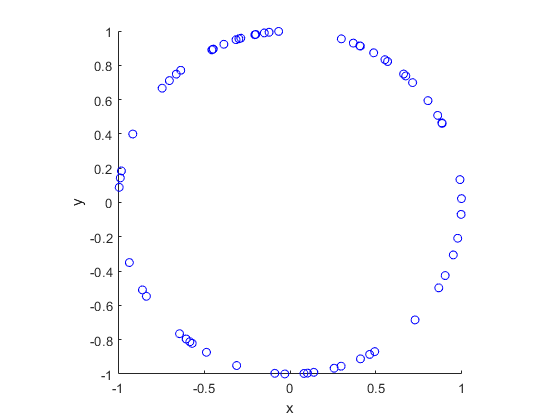
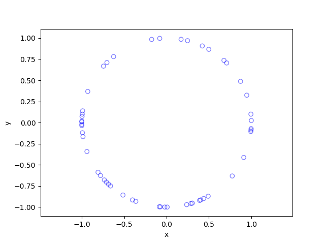
I have presented some results produced by code written in MATLAB and Python. The blue points are the Poisson points on the sphere. I have used a surface plot (with clear faces) in black to illustrate the underling sphere.

MATLAB

Python

Code

The code for all my posts is located online here. For this post, the code in MATLAB and Python is here.