Exponential distribution Archives

The inverse method for simulating random variables

We will cover a simple but much used method for simulating random variables or, rather, random variates. Although the material here is found in introductory probability courses, it frequently forms the foundation of more advance stochastic simulation techniques, such as Markov chain Monte Carlo methods.

Details

The basics of probability theory tell us that any random variable can, in theory, be written as a function of a uniform random variable $U$ distributed on the interval $(0,1)$, which is usually written as $U\sim U(0,1)$. All one needs is the inverse of the cumulative distribution function of the desired random variable.

More specifically, let $X$ be a random variable with a cumulative distribution function $F(x)=\mathbb{P}(X\leq x)$. The function $F$ is nondecreasing in $x$, so its inverse can be defined as $F^{-1}(y)=\inf\{x:F(x)\geq y\}$, which is known as the generalized inverse of $F(x)$.

Some authors assume the minimum is attained so the infimum is replaced with the minimum, giving $F^{-1}(y)=\min\{x:F(x)\geq y\}$.

In short, the following result is all that we need.

Transform of a uniform variable $U\sim U(0,1)$

For a uniform random variable $U\sim U(0,1)$, the random variable $F^{-1}(U)$ has the cumulative distribution function $\mathbb{P}(F^{-1}(U)\leq x)=P(U\leq F(x))=F(x)$.

Algorithm

The above observation gives a method, which I like to call the direct method, for exactly simulating a random variable $X$ with the (cumulative) distribution (function) $F$.

Random variable $X$ with distribution $F$

Sample a uniform random variable $U\sim U(0,1)$, giving a value $u$.

Return the value $x=F^{-1}(u)$ as the sampled value of $U$.

But this approach only works if we can write down (in a relatively straightforward way) the inverse $F^{-1}$, which is usually not the case. This means you cannot generate, for example, simulate a normal random variable with a single uniform random variable by using just the inverse method, as we cannot write down the inverse of its cumulative distribution function.

(Interestingly, with two (independent) uniform random variables, we can use the transform method to simulate two (independent) normal (or Gaussian) random variables. This approach is called the Box-Muller transform, which I’ll cover in another post.)

Nevertheless, we can apply the inverse method to some useful distributions.

Examples

Warning: The following examples are only for illustration purposes. Except for the Bernoulli example, you would never use them in standard scientific languages such as MATLAB, Python (with NumPy), R or Julia, because those languages already have much better functions for simulating these and many other random variables (or variates). If you are writing a function in a language that lacks such functions, I would consult one of the references mentioned below. Although the inverse method is usually intuitive and elegant, it is often not the fastest method.

Bernoulli distribution

The simplest random variable is that with the Bernoulli distribution. With probability $p$, a Bernoulli random variable $X$ takes the value one. Otherwise, $X$ takes the value zero (with probability $1-p$). This gives the (cumulative) distribution (function):

$$ F_B(x)=\begin{cases}
0 & \text{if } x < 0 \\
1 – p & \text{if } 0 \leq x < 1 \\
1 & \text{if } x \geq 1
\end{cases}$$

This gives a very simple way to simulate (or sample) a Bernoulli variable $X$ with parameter $p$.

Bernoulli random variable $X$ with parameter $p$

Sample a uniform random variable $U\sim U(0,1)$, giving a value $u$.

If $u\leq p$, return $x=1$; otherwise return $x=0$.

Application: Acceptance simulation methods

In random simulation code, whenever you do something (or not) with some probability $p$ (or probability $1-p$), then the code will perform the above step. Consequently, you see this in the (pseudo-)code of many stochastic simulations with random binary choices, particularly schemes that have an acceptance step such the Metropolis-Hastings method and other Markov chain Monte Carlo (MCMC) methods.

In MCMC schemes, a random (binary) choice is proposed and it is accepted with a certain probability, say, $\alpha $. This is the equivalent of accepting the proposed choice if some uniform random variable $U$ meets the condition $U\leq \alpha$.

This explains why the pseudo-code of the same algorithm can vary. Some pseudo-code will say accept with probability $\alpha$, while other pseudo-code will say do if $U\leq \alpha$. It’s two equivalent formulations.

Exponential distribution

The cumulative distribution function of an exponential variable with mean $1/\lambda$ is $F_E(x)= 1-e^{-\lambda x}$, which has the inverse $F^{-1}_E(y)=-(1/\mu)\ln[1-y]$. We can use the fact that on the interval $(0,1)$, a uniform variable $U\sim U(0,1)$ and $1-U$ have the same distribution. Consequently, the random variables $\ln [1-U]$ and $\ln U$ are equal in distribution.

This gives a method for simulating exponential random variables.

Exponential random variable $X$ with mean $1/\lambda$

Sample a uniform random variable $U\sim U(0,1)$, giving a value $u$.

Return $x=-(1/\lambda)\ln u$.

Application: Poisson simulation method

Of course you can use this method to simulate exponential random variables, but it has another application. In a previous post on simulating Poisson variables, I mentioned that exponential random variables can be used to simulate a Poisson random variable in a direct (or exact) manner. That method is based on the distances between the points of a homogeneous Poisson point process (on the real line) being exponential random variables.

But this method is only suitable for low values of $\lambda$, less than say fifteen.

Rayleigh distribution

The Rayleigh distribution is $\mathbb{P}(X\leq x)= (x/\sigma^2)e^{-x^2/(2\sigma^2)}$, where $\sigma>0$ is its scale parameter. The square root of an exponential variable with mean $1/\lambda$ has a Rayleigh distribution with scale parameter $\sigma=1/\sqrt{2\lambda}$.

Consequently, the generation method is similar to the previous example.

Rayleigh random variable $Y$ with scale parameter $\sigma>0$

Sample a uniform random variable $U\sim U(0,1)$, giving a value $u$.

Return $y=\sigma\sqrt{-2\ln u}$.

Other methods

The inverse method is intuitive and often succinct. But most functions for simulating random variables (or, more correctly, generating random variates) do not use these methods, as they are not fast under certain parameter regimes, such as large means. Consequently, other method are used such as approximations (with, say, normal random variables), such as the ones I outlined in this post on simulating Poisson random variables.

More complicated random systems, such as collections of dependent variables, can be simulated using Markov chain Monte Carlo methods, which is the direction we’ll take in a couple posts after this one.

Poisson (stochastic) process

One of the most important stochastic processes is Poisson stochastic process, often called simply the Poisson process. In a previous post I gave the definition of a stochastic process (also called a random process) alongside some examples of this important random object, including counting processes. The Poisson (stochastic) process is a counting process. This continuous-time stochastic process is a highly studied and used object. It plays a key role in different probability fields, particularly those focused on stochastic processes such as stochastic calculus (with jumps) and the theories of Markov processes, queueing, point processes (on the real line), and Levy processes.

The points in time when a Poisson stochastic process increases form a Poisson point process on the real line. In this setting the stochastic process and the point process can be considered two interpretations of the same random object. The Poisson point process is often just called the Poisson process, but a Poisson point process can be defined on more generals spaces. In some literature, such as the theory of Lévy processes, a Poisson point process is called a Poisson random measure, differentiating the Poisson point process from the Poisson stochastic process. Due to the connection with the Poisson distribution, the two mathematical objects are named after Simeon Poisson, but he never studied these random objects.

The other important stochastic process is the Wiener process or Brownian (motion process), which I cover in another post. The Wiener process is arguably the most important stochastic process. I have written that post and the current one with the same structure and style, reflecting and emphasizing the similarities between these two fundamental stochastic process.

In this post I will give a definition of the homogenous Poisson process. I will also describe some of its key properties and importance. In future posts I will cover the history and generalizations of this stochastic process.

Definition

In the stochastic processes literature there are different definitions of the Poisson process. These depend on the settings such as the level of mathematical rigour. I give a mathematical definition which captures the main characteristics of this stochastic process.

Definition: Homogeneous Poisson (stochastic) process

An integer-valued stochastic process $\{N_t:t\geq 0 \}$ defined on a probability space $(\Omega,\mathcal{A},\mathbb{P})$ is a homogeneous Poisson (stochastic) process if it has the following properties:

The initial value of the stochastic process $\{N_t:t\geq 0 \}$ is zero with probability one, meaning $P(N_0=0)=1$.

The increment $N_t-N_s$ is independent of the past, that is, $N_u$, where $0\leq u\leq s$.

The increment $N_t-N_s$ is a Poisson variable with mean $\lambda (t-s)$.

In some literature, the initial value of the stochastic process may not be given. Alternatively, it is simply stated as $N_0=0$ instead of the more precise (probabilistic) statement given above.

Also, some definitions of this stochastic process include an extra property or two. For example, from the above definition, we can infer that increments of the homogeneous Poisson process are stationary due to the properties of the Poisson distribution. But a definition may include something like the following property, which explicitly states that this stochastic process is stationary.

For $0\leq u\leq s$, the increment $N_t-N_s$ is equal in distribution to $N_{t-s}$.

The definitions may also describe the continuity of the realizations of the stochastic process, known as sample paths, which we will cover in the next section.

It’s interesting to compare these defining properties with the corresponding ones of the standard Wiener stochastic process. Both stochastic processes build upon divisible probability distributions. Using this property, Lévy processes generalize these two stochastic processes.

Properties

The definition of the Poisson (stochastic) process means that it has stationary and independent increments. These are arguably the most important properties as they lead to the great tractability of this stochastic process. The increments are Poisson random variables, implying they can have only positive (integer) values.

The Poisson (stochastic) process exhibits closure properties, meaning you apply certain operations, you get another Poisson (stochastic) process. For example, if we sum two independent Poisson processes $X= \{X_t:t\geq 0 \}$ and $Y= \{Y_t:t\geq 0 \}$, then the resulting stochastic process $Z=Z+Y = \{N_t:t\geq 0 \}$ is also a Poisson (stochastic) process. Such properties are useful for proving mathematical results.

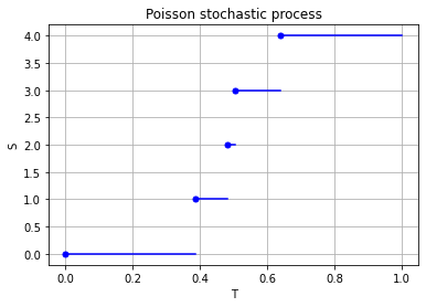
A single realization of a (homogeneous) Poisson stochastic process, where the blue marks show where the process jumps to the next value. In any finite time interval, there are a finite number of jumps.

Properties such as independence and stationarity of the increments are so-called distributional properties. But the sample paths of this stochastic process are also interesting. A sample path of a Poisson stochastic process is almost surely non-decreasing, being constant except for jumps of size one. (The term almost surely comes from measure theory, but it means with probability one.) There are only finitely number of jumps in each finite time interval.

The homogeneous Poisson (stochastic) process has the Markov property, making it an example of a Markov process. The homogenous Poisson process $N=\{ N_t\}_{t\geq 0}$s not a martingale. But interestingly, the stochastic process is $\{ W_t – \lambda t\}_{t\geq 0}$ is a martingale. (Such relations have been used to study such stochastic processes with tools from martingale theory.)

Stochastic or point process?

The Poisson (stochastic) process is a discrete-valued stochastic process in continuous time. The relation these types of stochastic processes and point process is a subtle one. For example, David Cox and Valerie Isham write on page 3 of their monograph:

The borderline between point processes and a number of other kinds of stochastic process is not sharply defined. In particular, any stochastic process in continuous time in which the sample paths are step functions, and therefore any any process with a discrete state space, is associated with a point process, where a point is a time of transition or, more generally, a time of entry into a pre-assigned state or set of states. Whether it is useful to look at a particular process in this way depends on the purpose of the analysis.

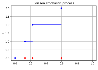
For the Poisson case, this association is presented in the diagram below. We can see the Poisson point process (in red) associated with the Poisson (stochastic) process (in blue) by simply looking at the time points where jumps occur.

A single realization of a (homogeneous) Poisson stochastic process (in blue). The jumps of the process form a (homogeneous) Poisson point process (in red) on the real line representing time.

Importance

Playing a prominent role in the theory of probability, the Poisson (stochastic) process is a highly important and studied stochastic process. It has connections to other stochastic processes and is central in queueing theory and random measures.

The Poisson process is a building block for more complex continuous-time Markov processes with discrete state spaces, which are used as mathematical models. It is also essential in the study of jump processes and subordinators.

The Poisson (stochastic) process is a member of some important families of stochastic processes, including Markov processes, Lévy processes, and birth-death processes. This stochastic process also has many applications. For example, it plays a central role in quantitative finance. It is also used in the physical sciences as well as some branches of social sciences, as a mathematical model for various random phenomena.

Generalizations and modifications

For the Poisson (stochastic) process, the index set and state space are respectively the non-negative numbers and counting numbers, that is $T=[0,\infty)$ and $S=0, 1, \dots$, so it has a continuous index set but a discrete state space. Consequently, changing the state space, index set, or both offers an ways for generalizing and modifying the Poisson (stochastic) process.

Simulation

The defining properties of the Poisson stochastic process, namely independence and stationarity of increments, results in it being easy to simulate. The Poisson stochastic process can be simulated provided random variables can be simulated or sampled according to a Poisson distributions, which I have covered in this and this post.

Simulating a Poisson stochastic process is similar to simulating a Poisson point process. (Basically, it is the same method in a one-dimensional setting.) But I will leave the details of sampling this stochastic process for another post.

Simulating Poisson random variables in Fortran

The hint’s in the title. I wrote a simple function in Fortran for simulating (or sampling) Poisson random variables. (More precisely, I should say that the function generates Poisson variates.) I used the simple direct method. This method is based on the exponential inter-arrival times of the Poisson (stochastic) process.

My code should not be used for large Poisson parameter values (larger than, say, 20 or 30), as the code may be too slow. Other methods exist for larger parameter values, which I’ve discussed previously.

I just use the standard Fortran function random_number for generating (pseudo-)random numbers. I am not an expert in Fortran, but my Poisson function seems to work fine. I wrote and ran a simple test that estimates the first and second moments, which should match for Poisson variables.

My Fortran code is very similar to the code that I wrote in C and C#, which is located here. You should be able to run it on this website or similar ones that can compile Fortran (95) code.

Code

On this page I’ve only included the code of the functions for generating uniform and Poisson variates. The rest of the code, including the test, is located here.

!Poisson function -- returns a single Poisson random variable
function funPoissonSingle(lambda) result(randPoisson)
real, intent(in) :: lambda !input
real :: exp_lambda !constant for terminating loop
real :: randUni !uniform variable
real :: prodUni !product of uniform variables
integer :: randPoisson !Poisson variable

exp_lambda= exp(-lambda) 

!initialize variables
randPoisson = -1;
prodUni = 1;
do while (prodUni > exp_lambda)
   randUni = funUniformSingle() !generate uniform variable
   prodUni = prodUni * randUni; !update product
   randPoisson = randPoisson + 1 !increase Poisson variable
end do
end function

!Uniform function -- returns a standard uniform random variable
function funUniformSingle() result(randUni)
real randUni;
call random_seed
call random_number(randUni)

end function

The Standard Model of wireless networks

In the previous post I discussed the signal-to-interference-plus ratio or SIR in wireless networks. If noise is included, then then signal-to-interference-plus-noise ratio or just SINR. But I will just write about SIR, as most results that hold for SIR, will also hold for SINR without any great mathematical difficulty.

The SIR is an important quantity due to reasons coming from information theory. If you’re unfamiliar with it, I suggest reading the previous post.

In this post, I will describe a very popular mathematical model of the SIR, which I like to call the standard model. (This is not a term used in the literature as I have borrowed it from physics.)

Definition of SIR

To define the SIR, we consider a wireless network of $n$ transmitters with positions located at $X_1,\dots,X_n$ in some region of space. At some location $x$, we write $P_i(x)$ to denote the power value of a signal received at $x$ from transmitter $X_i$. Then at location $x$, the SIR with respect to transmitter $X_i$ is
$$
\text{SIR}(x,X_i) := \frac{P_i(x)}{\sum\limits_{j\neq i} P_j(x)} .
$$

Researchers usually attempt to represent the received power of the signal $P_i(x)$ with a propagation model. This mathematical model consists of a random and a deterministic component given by
$$
P_i(x)=F_i\ell(|X_i-x|) ,
$$
where $\ell(r)$ is a non-negative function in $r\geq 0$ and $F_i$ is a non-negative random variable. The function $\ell(r)$ is often called the path loss function. The random variables represent random fading or shadowing.

Standard model

Based on the three model components of fading, path loss, and transmitter locations, there are many combinations possible. That said, researchers generally (I would guess, say, 90 percent or more) use a single combination, which I call the standard model.

The three standard model assumptions are:

Singular power law path loss $\ell(r)=(\kappa r)^{-\beta}$.
Exponential distribution for fading variables, which are independent and identically distributed (iid).
Poisson point process for transmitter locations.

Why these three? Well, in short, because they work very well together. Incredibly, it’s sometimes possible to get relatively a simple mathematical expression for, say, the coverage probability $\mathbb{P}[\text{SIR}(x,X_i)>\tau ]$, where $\tau>0$.

I’ll now detail the reasons more specifically.

Path loss

The $\ell(r)=(\kappa r)^{-\beta}$ is very simple, despite having a singularity at $r=0$. This allows simple algebraic manipulation of equations.

Some, such as myself, are initially skeptical of this function as it gives an infinitely strong signal at the transmitter due to the singularity in the function $\ell(r)=(\kappa r)^{-\beta}$. More specifically, the path loss of the signal from transmitter $X_i$ approaches infinity as $x$ approaches $X_i$ .

But apparently, overall, the singularity does not have a significant impact on most mathematical results, at least qualitatively. That said, one still observe consequences of this somewhat physically unrealistic model assumption. And I strongly doubt enough care is taken by researchers to observe and note this.

Fading and shadowing variables

Interestingly, the original reason why exponential variables were used is because it allowed the SIR problem to be reformulated into a problem of a Laplace transform of a random variable, which for a random variable $Y$ is defined as

$$
\mathcal{L}_Y(t)=\mathbb{E}(e^{- Y t}) \, .
$$

where $t\geq 0$. (This is essentially the moment-generating function with $-t$ instead of $t$.)

The reason for this connection is that the tail distribution of an exponential variable $F$ with mean $\mu$ is simply $\mathbb{P}(F>t)= e^{-t/\mu}$. In short, with the exponential assumption, various conditioning arguments eventually lead to Laplace transforms of random variables.

Transmitters locations

No prizes for guessing that researcher overwhelmingly use a (homogeneous) Poisson point process for the transmitter (or receiver) locations. When developing mathematical models with point processes, if you can’t get any results with the Poisson point process, then abandon all hope.

It’s the easier to work with this point process due to its independence property, which leads to another useful property. For Poisson point process, the Palm distribution is known, which is the distribution of a point process conditioned on a point (or collection of points) existing in a specific location of the underlying space on which the point process is defined. In general, the Palm distribution is not known for many point processes.

Random propagation effects can lead to Poisson

A lesser known reason why researchers would use the Poisson point process is that, from the perspective of a single observer in the network, it can be used to capture the randomness in the signal strengths. Poisson approximation results in probability imply that randomly perturbing the signal strengths can make signals appear more Poisson, by which I mean the signal strengths behave stochastically or statistically as though they were created by a Poisson network of transmitters.

The end result is that a non-Poisson network can appear more Poisson, even if the transmitters do not resemble (the realization of) a Poisson point process. The source of randomness that makes a non-Poisson network appear more Poisson is the random propagation effects of fading, shadowing, randomly varying antenna gains, and so on, or some combination of these.

Simulating Poisson random variables – Survey of methods

In the previous post, I discussed how to sample or generate Poisson random variables or, more correctly, variates. I detailed a direct method that uses the fact that a Poisson stochastic process, which is directly related to a Poisson point process, has inter-arrival times that form independent and identically distributed exponential variables.

This direct method in turn can be easily reformulated so it only uses (standard) uniform variables to generate Poisson random variables. It is an easy and intuitive sampling method, explaining why it is often used. Using it, I wrote Poisson simulation code in MATLAB, Python, C and C#, which can be found here. (For another post, I later implemented the same Poisson sampling method in Fortran, which is located here.)

As elegant and exact as this simulation method is, it unfortunately decreases in speed as the Poisson parameter $\lambda$ increases. In a tutorial published in 1983, Brian D. Ripely, a major figure in spatial statistics, says this about the direct method:

This is simple, but has expected time proportional to $\lambda$. Some of its competitors use rejection methods with the envelope distribution that of the integer part of a continuous random variable, such as logistic, Laplace and normal mixed with exponential distributions.

We recall that acceptance-rejection or rejections methods involve simulating a random object, such as a random variable, by first simulating another random object of the same type that is easier to simulate. The simulation method then accepts or rejects these random objects based on a certain ratio. The distribution of the simpler random object that is first simulated is called the envelope distribution. Such rejection methods are one way to simulate Poisson variables.

In short, when simulating Poisson variables, the appropriate simulation algorithm should be chosen based on the Poisson parameter. Consequently, the code of most computer functions for generating Poisson variables will have an if-statement, using the direct method for small parameter values and another method for large parameter values. We now consider the other methods.

Different methods

Over the years there have been different methods proposed for producing Poisson random variates. In the book Non-uniform random variate generation, Luc Devroye groups the different methods into five categories coupled with his views. I’ll briefly describe these methods:

Direct methods based on the homogeneous Poisson stochastic process having exponential inter-arrival times. These methods are simple, but the expected time is proportional to the Poisson parameter $\lambda$.
Inversion methods that search through a table of cumulative Poisson probabilities. Examples include the papers by Fishman (1976) and Atkinson (1979)*.
Methods that use the recursive properties of the Poisson distribution. The paper by Ahrens and Dieter (1974) uses this approach, and its expected time of completion is proportional to $\log\lambda$.
Acceptance-rejection (or rejection) methods that give relatively fast but simple algorithms. Such methods are proposed in the papers by Atkinson (1979)*, Ahrens and Dieter (1980) and Devroye (1981) or the technical report by Schmeiser and Kachitvichyanukul (1981).
Acceptance-complement methods that uses a normal distribution as the starting distribution, such as the paper by Ahrens and Dieter (1982). This method is fast, but the code is rather long.

*Atkinson had (at least) two papers on generating Poisson variates published in 1979, but I believe Devroye is referring to the first paper, because in the second paper Atkinson compares methods proposed by others.

For the paper titles, see the Further reading section below.

Methods implemented

In this section, I’ll state which proposed methods are used in various programming languages and numerical methods. I won’t go into the details how the methods work, as I’ll just cite the papers instead.

MATLAB

For small $\lambda$ values, the MATLAB function poissrnd uses the direct method (based on inter-arrival times) with a while-loop.

For $\lambda$ values greater than fifteen, I believe that the MATLAB function poissrnd uses Algorithm PG from the 1974 paper by Ahrens and Dieter. But to come to this conclusion, I had to do some investigating. You can skip to the next section if you’re not interested, but now I’ll explain my reasoning.

The MATLAB documentation says it uses a method proposed by Ahrens and Dieter, but these two researchers developed a number of methods for generating Poisson variables. The MATLAB code cites Volume 2 of the classic series by Knuth, who says the method is due to Ahrens and Dieter, but he doesn’t give an exact citation in that section of the book. Confusingly, Knuth cites in his book a couple papers by Ahrens and Dieter for generating different random variates. (Knuth later cites a seemingly relevant 1980 paper by Ahrens and Dieter, but that details another method.)

Both the MATLAB code and Knuth cite the book by Devroye. In his book (Exercise 3.5.2), Devroye discusses one method, among others, from a 1974 paper by Ahrens and Dieter. Another hint is given by examining the code of the MATLAB function poissrnd, which reveals that it uses the function randg to generate gamma variables. In the Ahrens and Dieter 1974 paper, their Algorithm PG (for producing Poisson variates) uses gamma random variables, and it’s suggested to use a parameter value of $7/8$. This is the same parameter used in the MATLAB code and mentioned by Knuth, confirming that this is the right paper by Ahrens and Dieter.

In summary, for large $\lambda$ the function MATLAB uses Algorithm PG from the 1974 paper by Ahrens and Dieter, whereas for small values it uses the direct method, which they refer to as the multiplication method.

R

In R, the function rpois use an algorithm outlined in the 1982 paper by Ahrens and Dieter. You can view the R source code here. The two cases for $\lambda$ (or $\mu$ in the paper) depend on whether $\lambda$ is greater than ten or not. For small $\lambda$, the R function rpois does not use the method based on inter-arrival times, but rather an inversion method based on a table of (cumulative) probabilities given by the Poisson probability distribution.

Python (NumPy)

In NumPy, the function numpy.random.poisson generates Poisson variates. The source code for the NumPy library is here, but for the Poisson function the underlying code is actually written in C; see the distributions.c file located here. For small Poisson parameter $\lambda$, the code uses the direct method; see the function random_poisson_mult in the code.

For Poisson parameter $\lambda \geq 10$, the comments in the code reveal that it uses a method from a 1993 paper by Hörmann; see Algorithm PTRS on page 43 of the paper. This is a transformation method, which for NumPy is implemented in the C code as the function random_poisson_ptrs. The method, which Hörmann calls the transformed rejection with squeeze, combines inversion and rejection methods.

Octave

Octave is intended to be a GNU clone of MATLAB, so you would suspect it uses the same methods as MATLAB for generating Poisson random variates. But the Octave function poissrnd uses different methods. The code reveals it generates the Poisson variates with a function called prand. It considers different cases depending on the value of the Poisson parameter $\lambda$ as well as whether a single variable (that is, a scalar) or vector or matrix of Poisson variates are being generated.

In total, the Octave function prand uses five different methods. For two of the methods, the documentation cites methods from the classic book Numerical Recipes in C (the 1992 edition); see next section. To generate a single Poisson variate with Poisson parameter $\lambda \leq 12$, the Octave function prand uses the direct method based on inter-arrival times.

Numerical Recipes (Fortran, C and C++)

The book Numerical Recipes is a classic by Press, Teukolsky, Vetterling and Flannery on numerical methods. The books comes in different editions reflecting different publication years and computer languages. (In the first two editions of the book, the authors implemented the algorithms respectively in Fortran and C.)

For generating Poisson variates, the book contents seems to have not changed over the editions that I looked at, which covered the programming languages Fortran (77 and 90), C, and C++. The authors cover Poisson generation in Section 7.3 in the Fortran and C editions. In the third edition of Numerical Recipes, they implement their methods in C++ in Section 7.3.12.

For small values of Poisson parameter $\lambda$, Numerical Recipes uses the direct method. For $\lambda >12$ values, an acceptance-rejection method is used, which relies upon finding a continuous version of the discrete Poisson probability distribution.

GSL Library (C)

In the GSL library, one can use the function gsl_ran_poisson, which uses the the direct method of exponential times. The code, which can be viewed here, cites simply Knuth (presumably the second volume).

NAG Library (C)

Although I didn’t see the code, it appears that the function nag_rand_poisson (g05tjc ) in the NAG library also uses the direct method, based on the material in the second volume of series by Knuth. But in a 1979 paper Atkinson says that the NAG library uses a method from the 1974 paper by Ahrens and Dieter.

MKL library (C)

In the MKL C library written by Intel, there seems to be three methods in use for generating Poisson variates.

The first function is called VSL_RNG_METHOD_POISSON_PTPE, which does the following for a Poisson distribution with parameter $\Lambda$:

If Λ ≥ 27, random numbers are generated by PTPE method. Otherwise, a combination of inverse transformation and table lookup methods is used. The PTPE method is a variation of the acceptance/rejection method that uses linear (on the fraction close to the distribution mode) and exponential (at the distribution tails) functions as majorizing functions. To avoid time-consuming acceptance/rejection checks, areas with zero probability of rejection are introduced and a squeezing technique is applied.

This function uses the so-called PTPE method, which is outlined in a 1981 technical report by Schmeiser and Kachitvichyanukul.

The second function is called VSL_RNG_METHOD_POISSON_POISNORM, which does the following :

If Λ < 1, the random numbers are generated by combination of inverse transformation and table lookup methods. Otherwise, they are produced through transformation of the normally distributed random numbers.

The third function is called VSL_RNG_METHOD_POISSONV_POISNORM, which does the following:

If Λ < 0.0625, the random numbers are generated by inverse transformation method. Otherwise, they are produced through transformation of normally distributed random numbers.

cuRAND (C)

Finally, Nvidia’s CUDA Random Number Generation library (cuRAND) has a function for generating Poisson variates. To see the C code, copies of it can be found in various GitHub repositories, such as this one. The cuRAND function curand_poisson uses the direct function for Poisson parameter values less than 64. For parameters values greater than 4000, it uses a normal approximation (rounded to the nearest integer).

For other values, the function curand_poisson uses a rejection method based on an approximation of the incomplete gamma function; see the function curand_poisson_gammainc. The book by Fishman is cited; see Section 8.16.

Boost library Random (C++)

The Boost library Random uses the PTRD algorithm proposed in the 1993 paper by Hörmann to generate Poisson variates; see Algorithm PTRD on page 42 of the paper. In the same paper appears the PTRS method, which is used by Python (NumPy) (though implemented in C), as mentioned above.

Simulating Poisson random variables – Direct method

If you were to write from scratch a program that simulates a homogeneous Poisson point process, the trickiest part would be the random number of points, which requires simulating a Poisson random variable. In previous posts, such as this one and this one, I’ve simply used the inbuilt functions for simulating (or generating) Poisson random variables (or variates).¹

But how would one create such a Poisson function using just a standard uniform random variate generator? In this post I will write my own Poisson simulation code in MATLAB, Python, C and C#, which can be found here.

The method being used depends on the value of the Poisson parameter, denoted here by $\lambda$, which is the mean (as well as the variance) of a random variable with a Poisson distribution. If this parameter value is small, then a direct simulation method can be used to generate Poisson random variates. In practice a small Poisson parameter is a number less than some number between 10 to 30.

For large $\lambda$ values, other methods are generally used, such as rejection or (highly accurate) approximation methods. In the book Non-uniform random variate generation, the author Luc Devroye groups the methods into five categories (Section X.3.2), which I briefly describe in the next post. The first of those categories covers the method that I mentioned above. I will cover that method in this post, presenting some Poisson sampling code in C and C#. (I will also present some code in MATLAB, but you would never use it instead of the the inbuilt function poissrnd.)

In the next post, I’ll describe other types of Poisson simulation methods, and I’ll detail which simulation methods various programming libraries use.

Warning: My online webpage editor tends to mangle symbols like < and >, so it’s best not to copy my code straight from the website, unless you check and edit it.

Direct method

An elegant and natural method for simulating Poisson variates is to a result based on the homogeneous Poisson stochastic process. The points in time when a given homogeneous Poisson stochastic process increases forms a Poisson point process on the real line. ²

Using exponential random variables

Here’s the algorithm for sampling Poisson variables with exponential random variables, which I’ll explain.

Sample Poisson random variable $N$ with parameter (mean) $\lambda$ using exponential random variables

Set count variable $N=0$ and initial sum variable $S=0$;

While $S<1$:

Sample uniform random variable $U\sim U(0,1)$;

Calculate $E= -\log(U)/\lambda $ ;

Update count and sum variables by setting $N\rightarrow N+1$ and $S\rightarrow S+E$;

Return N;

The point in time when the Poisson stochastic process increases are called arrival times or occurrence times. In classic random models they represent the arrivals or occurrences of something, such as phone calls over time. The differences between consecutive times are called inter-arrival times or inter-occurrence times. The inter-arrival times of a homogeneous Poisson process form independent exponential random variables, a result known as the Interval Theorem.

Using this connection to the Poisson stochastic process, we can generate exponential variables $E_1$, $E_2, \dots $, and add them up. The smallest number of exponential variables for the resulting sum to exceeds one will give a Poisson random variable. That is, if we define $N$ to be the smallest $n$ such that
$$ \sum_{k=1}^{n+1} E_k > 1, $$
then $N$ is a random variable distributed according to a Poisson distribution.

Generating exponential variates is easily done by using the inverse method. For a uniform random variable $U$ on the unit interval $(0,1)$, the transformation $E= -\log(U)/\lambda $ gives an exponential random variable with mean $1/\lambda$.

But we can skip generating exponential random variates.

Using uniform random variables

Here’s the algorithm for sampling Poisson variables with uniform random variables.

Sample Poisson random variable $N$ with parameter (mean) $\lambda$ using uniform random variables

Set count variable $N=0$ and initial product variable $P=1$;

While $P>e^{-\lambda}$:

Sample uniform random variable $U\sim U(0,1)$;

Update count and product variables by setting $N\rightarrow N+1$ and $P\rightarrow P\times U$;

Return N;

To reduce computations, the direct method using exponential random variables is often reformulated as products of uniform random variables. We can do this, due to logarithmic identities, and work with products of uniform variables instead of sums of exponential random variables.

Then, by using standard uniform random variables $U_1, U_2,\dots$, we define $N$ to be the smallest $n$ such that
$$ \prod_{k=1}^{n+1} U_k < e^{-\lambda}. $$

These two different formulations of the same method are captured by Lemma 3.2 and Lemma 3.3 in Chapter 10 of Devroye’s book.

Example in MATLAB

In MATLAB, we can implement this method with the first formulation in a function with a simple while-loop:

function N=funPoissonLoop(lambda)
T=0; %initialize sum of exponential variables as zero
n=-1;%initialize counting variable as negative one

while (T <1)
E=-(1/lambda)*log(rand(1));%generate exponential random variable
T=T+E; %update sum of exponential variables
n=n+1; %update number of exponential variables
end
N=n;
end

But, as I said before, don’t use this code instead of the inbuilt function poissrnd.

If you want to be a bit more tricky, you could achieve the same result by using recursion:

function N=funPoissonRecursive(lambda)
T=0; %initialize sum of exponential variables as zero
n=-1; %initialize counting variable as negative one

%run (recursive) exponential function step function
[~,N]=funStepExp(lambda,T,n);

function [T,N]=funStepExp(nu,S,m)
if (S < 1)
%run if sum of exponential variables is not high enough

%generate exponential random variable
E=(-log(rand(1)))/nu;
S=S+E; %update sum of exponential variables
m=m+1; %update nunber of exponential variables

%recursively call function again
[T,N]=funStepExp(nu,S,m);
else
T=S;
N=m;
end
end
end

Note how the code recursively calls the function funStepExp, which generates an exponential variable each time.

In the Code section below I describe my code in C and C#, using the second formulation.

Origins

Some people attribute the direct method, based on inter-arrival times, to (or, at least, cite) Donald Knuth, who details it in the second volume of his classic series of books, but I doubt that the great Knuth was the first to have this idea. For example, a quick search on Google Scholar found a paper by K. D. Tocher on computers and random sampling, where Tocher proposes the direct method in 1954, some years before Knuth started publishing his classic series.

The direct method for Poisson sampling relies upon the Interval theorem. The Poisson point process expert Günter Last studied the origins of this fundamental result. He presented its history in a recent book authored by him and Matthew Penrose; see Chapter 7 and its corresponding historical footnotes in Section C of the appendix. (A free version of the book can be found here. ) People connected to the result include Robert Ellis and William Feller.

Other methods

The direct method perfectly generates Poisson random variables (or I should say Poisson random variates). But it can be too slow for large values of the Poisson parameter (that, is the mean) $\lambda$. This has motivated researchers to develop other methods, which I will mention in the next post.

Code

I wrote some code that simulates Poisson random variables by employing the direct method based on exponential inter-arrival times. As always, all my the code is online, with the code from this post being located here.

I have implemented the second formulation (using just uniform variables) in the C and C# languages. In the code, I have used a while-loop to implement the method. But I could have also used a recursion method, as I did in the MATLAB example above, which I have also done in Python (with NumPy).

For an empirical test, the code also calculates the mean and variance of a collection of Poisson variables. For a large enough number of variables, the sample mean and the variance will closely agree with each other, converging to the same value.

C

Warning: My C code uses rand(), the standard pseudo-random number function in C, which is known for failing certain tests of randomness. The function is adequate for regular simulation work. But it gives poor results for large number of simulations. Replace this function with another pseudo-random number generator.

The code for generating a single Poisson variate is fairly straightforward in C. Here’s a sample of the code with just the Poisson function:

//Poisson function -- returns a single Poisson random variable
int funPoissonSingle(double lambda)
{
double exp_lambda = exp(-lambda); //constant for terminating loop
double randUni; //uniform variable
double prodUni; //product of uniform variables
int randPoisson; //Poisson variable

//initialize variables
randPoisson = -1;
prodUni = 1;
do
{
randUni = funUniformSingle(); //generate uniform variable
prodUni = prodUni * randUni; //update product
randPoisson++; //increase Poisson variable

} while (prodUni > exp_lambda);
return randPoisson;
}

For generating multiple variates, the code becomes more complicated, as one needs to use pointers, due to the memory capabilities of C. Again, the function uses the pseudo-random number generator in C.

C#

The code for generating a single Poisson variate is also straightforward in C#. Here’s the function in C#:

//Poisson function -- returns a single Poisson random variable
public int funPoissonSingle (double lambda) {
double exp_lambda = Math.Exp (-lambda); //constant for terminating loop
double randUni; //uniform variable
double prodUni; //product of uniform variables
int randPoisson; //Poisson variable

//initialize variables
randPoisson = -1;
prodUni = 1;
do {
randUni = funUniformSingle (); //generate uniform variable
prodUni = prodUni * randUni; //update product
randPoisson++; // increase Poisson variable

} while (prodUni > exp_lambda);

return randPoisson;
}

Generalizing the code so it generates multiple variates just requires a little change, compared to C, as the C# language is a much more modern language.

Fortran

After this original post, I later wrote a post about implementing the same Poisson algorithm in Fortran. My Fortran code is very similar to the code that I wrote in C and C#. You should be able to run it on this website or similar ones that can compile Fortran (95) code.

Details

Algorithm

Examples

Bernoulli distribution

Application: Acceptance simulation methods

Exponential distribution

Application: Poisson simulation method

Rayleigh distribution

Other methods

Further reading

Definition

Properties

Stochastic or point process?

Importance

Generalizations and modifications

Simulation

Further reading

Further reading

Code

Definition of SIR

Standard model

Path loss

Fading and shadowing variables

Transmitters locations

Random propagation effects can lead to Poisson

Further reading

Different methods

Methods implemented

MATLAB

R

Python (NumPy)

Octave

Numerical Recipes (Fortran, C and C++)

GSL Library (C)

NAG Library (C)

MKL library (C)

cuRAND (C)

Boost library Random (C++)

Further reading

Books

Articles

Direct method

Using exponential random variables

Sample Poisson random variable \(N\) with parameter (mean) \(\lambda\) using exponential random variables

Using uniform random variables

Sample Poisson random variable \(N\) with parameter (mean) \(\lambda\) using uniform random variables

Example in MATLAB

Origins

Other methods

Code

C

C#

Fortran

Further reading