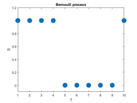
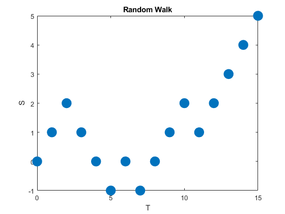
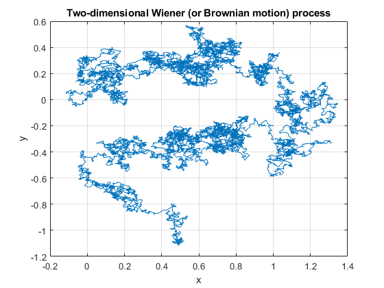
One of the most important stochastic processes is the Wiener process or Brownian (motion) process. In a previous post I gave the definition of a stochastic process (also called a random process) with some examples of this important random object, including random walks. The Wiener process can be considered a continuous version of the simple random walk. This continuous-time stochastic process is a highly studied and used object. It plays a key role different probability fields, particularly those focused on stochastic processes such as stochastic calculus and the theories of Markov processes, martingales, Gaussian processes, and Levy processes.
The Wiener process is named after Norbert Wiener, but it is called the Brownian motion process or often just Brownian motion due to its historical connection as a model for Brownian movement in liquids, a physical phenomenon observed by Robert Brown. But the physical process is not true a Wiener process, which can be treated as an idealized model. I will use the terms Wiener process or Brownian (motion) process to differentiate the stochastic process from the physical phenomenon known as Brownian movement or Brownian process.
The Wiener process is arguably the most important stochastic process. The other important stochastic process is the Poisson (stochastic) process, which I cover in another post. I have written that and the current post with the same structure and style, reflecting and emphasizing the similarities between these two fundamental stochastic process.
In this post I will give a definition of the standard Wiener process. I will also describe some of its key properties and importance. In future posts I will cover the history and generalizations of this stochastic process.
Definition
In the stochastic processes literature there are different definitions of the Wiener process. These depend on the settings such as the level of mathematical rigour. I give a mathematical definition which captures the main characteristics of this stochastic process.
Definition: Standard Wiener or Brownian (motion) process
A real-valued stochastic process \(\{W_t:t\geq 0 \}\) defined on a probability space \((\Omega,\mathcal{A},\mathbb{P})\) is a standard Wiener (or Brownian motion) process if it has the following properties:
- The initial value of the stochastic process \(\{W_t:t\geq 0 \}\) is zero with probability one, meaning \(P(W_0=0)=1\).
- The increment \(W_t-W_s\) is independent of the past, that is, \(W_u\), where \(0\leq u\leq s\).
- The increment \(W_t-W_s\) is a normal variable with mean \(o\) and variance \(t-s\).
In some literature, the initial value of the stochastic process may not be given. Alternatively, it is simply stated as \(W_0=0\) instead of the more precise (probabilistic) statement given above.
Also, some definitions of this stochastic process include an extra property or two. For example, from the above definition, we can infer that increments of the standard Wiener process are stationary due to the properties of the normal distribution. But a definition may include something like the following property, which explicitly states that this stochastic process is stationary.
- For \(0\leq u\leq s\), the increment \(W_t-W_s\) is equal in distribution to \(W_{t-s}\).
The definitions may also describe the continuity of the realizations of the stochastic process, known as sample paths, which we will cover in the next section.
It’s interesting to compare these defining properties with the corresponding ones of the homogeneous Poisson stochastic process. Both stochastic processes build upon divisible probability distributions. Using this property, Lévy processes generalize these two stochastic processes.
Properties
The definition of the Wiener process means that it has stationary and independent increments. These are arguably the most important properties as they lead to the great tractability of this stochastic process. The increments are normal random variables, implying they can have both positive and negative (real) values.
The Wiener process exhibits closure properties, meaning you apply certain operations, you get another Wiener process. For example, if \(W= \{W_t:t\geq 0 \}\) is a Wiener process, then for a scaling constant \(c>0\), the resulting stochastic process \(\{W_{ct}/\sqrt{c}:t \geq 0 \}\)is also a Wiener process. Such properties are useful for proving mathematical results.
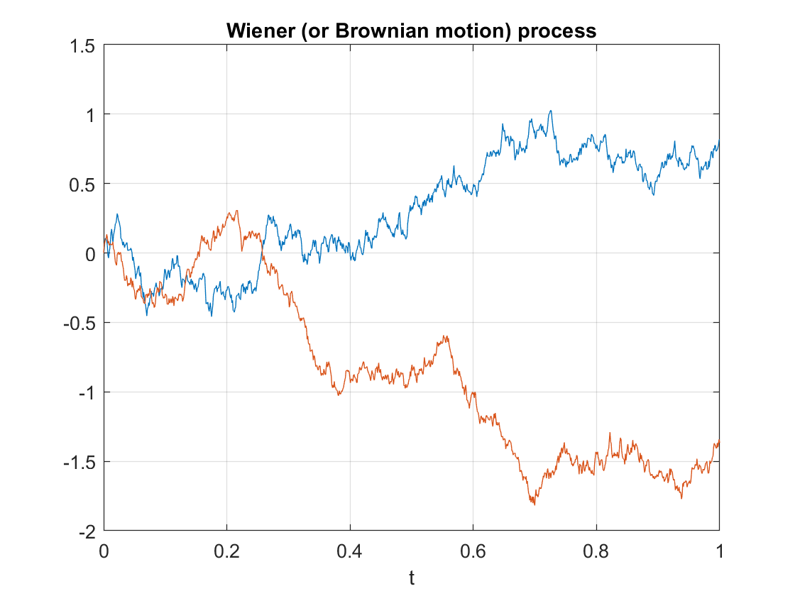
Properties such as independence and stationarity of the increments are so-called distributional properties. But the sample paths of this stochastic process are also interesting. A sample path of a Wiener process is continuous almost everywhere. (The term almost everywhere comes from measure theory, but it simply means that the only region where the property does not hold is mathematically negligible.) Despite the continuity of the sample paths, they are nowhere differentiable. (Historically, it was a challenge to find such a function, but a classic example is the Weierstrass function.)
The standard Wiener process has the Markov property, making it an example of a Markov process. The standard Wiener process \(W=\{ W_t\}_{t\geq 0}\) is a martingale. Interestingly, the stochastic process \(W=\{ W_t^2-t\}_{t\geq 0}\) is also a martingale. The Wiener process is a fundamental object in martingale theory.
There are many other properties of the Brownian motion process; see the Further reading section for, well, further reading.
Importance
Playing a main role in the theory of probability, the Wiener process is considered the most important and studied stochastic process. It has connections to other stochastic processes and is central in stochastic calculus and martingales. Its discovery led to the development to a family of Markov processes known as diffusion processes.
The Wiener process also arises as the mathematical limit of other stochastic processes such as random walks, which is the subject of Donsker’s theorem or invariance principle, also known as the functional central limit theorem.
The Wiener process is a member of some important families of stochastic processes, including Markov processes, Lévy processes, and Gaussian processes. This stochastic process also has many applications. For example, it plays a central role in quantitative finance. It is also used in the physical sciences as well as some branches of social sciences, as a mathematical model for various random phenomena.
Generalizations and modifications
For the Brownian motion process, the index set and state space are respectively the non-negative numbers and real numbers, that is \(T=[0,\infty)\) and \(S=[0,\infty)\), so it has both continuous index set and state space. Consequently, changing the state space, index set, or both offers an ways for generalizing or modifying the Wiener (stochastic) process.
Simulating
The defining properties of the Wiener process, namely independence and stationarity of increments, results in it being easy to simulate. The Wiener can be simulated provided random variables can be simulated or sampled according to a normal distribution. The main challenge is that the Wiener process is a continuous-time stochastic process, but computer simulations run in a discrete universe.
I will leave the details of sampling this stochastic process for another post.
Further reading
A very quick history of Wiener process and the Poisson (point) process is covered in this talk by me.
There are books almost entirely dedicated to the subject of the Wiener or Brownian (motion) process, including:
- Peres and Mörters, Brownian Motion
- Le Gall, Brownian Motion, Martingales, and Stochastic Calculus;
- Schilling and Partzsch, Brownian Motion: An Introduction to Stochastic Processes;
- Karatzas and Shreve, Brownian Motion and Stochastic Calculus.
Of course the stochastic process is also covered in any book on stochastic calculus:
- Klebaner, Introduction to Stochastic Calculus with Applications;
- Oksendal, Stochastic Differential Equations: An Introduction with Applications;
- Shreve, Stochastic Calculus for Finance II: Continuous-Time Models.
More advanced readers can read about the Wiener process, its descrete-valued cousin, the Poisson (stochastic) process, as well as other Lévy processes:
- Kyprianou, Fluctuations of Lévy Processes with Applications;
- Bertoin, Lévy Processes;
- Applebaum, Lévy Processes and Stochastic Calculus.
On this topic, I recommend the introductory article:
- 2004, Applebaum, Lévy Processes – From Probability to Finance and Quantum Groups.
The Wiener process is of course also covered in general books on stochastic process such as:
- Resnick, Adventures in Stochastic Processes;
- Parzen, Stochastic Processes;
- Durrett, Essentials of Stochastic Processes;
- Rosenthal, A First Look at Stochastic Processes.