

The binomial point process is arguably the simplest point process. It consists of a non-random number of points scattered randomly and independently over some bounded region of space. In this post I will describe the binomial point process, how it leads to the Poisson point process, and its historical role as stars in the sky.
The binomial point process is an important stepping stone in the theory of point process. But I stress that for mathematical models, I would always use a Poisson point process instead of a binomial one. The only exception would be if you were developing a model for a small, non-random number of points.
Uniform binomial point process
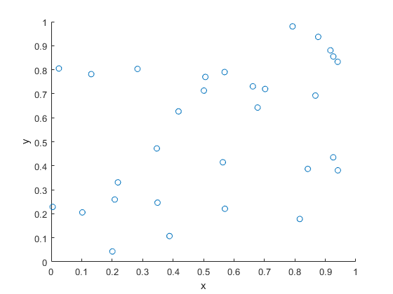
We start with the simplest binomial point process, which has uniformly located points. (I described simulating this point process in an early post. The code is here.)
Definition
Consider some bounded (or more precisely, compact) region, say, \(W\), of the plane plane \(\mathbb{R}^2\), but the space can be more general. The uniform binomial point process is created by scattering \(n\) points uniformly and independently across the set \(W\).
Distribution
Consider a single point uniformly scattered in the region \(W\), giving a binomial point process with \(n=1\). We look at some region \(B\), which is a subset of \(W\), implying \(B\subseteq W\). What is the probability that the single point \(X\) falls in region \(B\)?
First we write \(\nu(W)\) and \(\nu(B)\) to denote the respective areas (or more precisely, Lebesgue measures) of the regions \(W\) and \(B\), hence \(\nu(B)\leq \nu(W)\). Then this probability, say, \(p\), is simply the ratio of the two areas, giving
$$p= P(X\in B)=\frac{\nu(B)}{\nu(W)}.$$
The event of a single point being found in the set \(B\) is a single Bernoulli trial, like flipping a single coin. But if there are \(n\) points, then there are \(n\) Bernoulli trials, which bring us to the binomial distribution.
For a uniform binomial point process \(N_W\), the number of randomly located points being found in a region \(B\) is a binomial random variable, say, \(N_W(B)\), with probability parameter \(p=\nu(B)/ \nu(W)\). The probability mass function of \(N_W(B)\) is
$$ P(N_W(B)=k)={n\choose k} p^k(1-p)^{n-k}. $$
We can write the expression more explicitly
$$ P(N_W(B)=k)={n\choose k} \left[\frac{\nu(B)}{ \nu(W)}\right]^k\left[1-\frac{\nu(B)}{\nu(W)}\right]^{n-k}. $$
Poisson limit
Poisson random variable
A standard exercise in introductory probability is deriving the Poisson distribution by taking the limit of the binomial distribution. This is done by sending \(n\) (the total number of Bernoulli trials) to infinity while keeping the binomial mean \(\mu:=p n\) fixed, which sends the probability \(p=\mu/n\) to zero.
More precisely, for \(\mu\geq0\), setting \(p_n=\mu/n \) and keeping \(\mu :=p_n n\) fixed, we have the limit result
$$\lim_{n\to \infty} {n \choose k} p_n^k (1-p_n)^{n-k} = \frac{\mu^k}{k!}\, e^{-\mu}.$$
We can use, for example, Stirling’s approximation to prove this limit result.
We can make the same limit argument with the binomial point process.
Homogeneous Poisson point process
We consider the intensity of the uniform binomial point process, which is the average number of points in a unit area. For a binomial point process, this is simply
$$\lambda := \frac{n}{\nu(W)}.$$
For the Poisson limit, we expand the region \(W\) so it covers the whole plane \(\mathbb{R}^2\), while keeping the intensity \(\lambda = n/\nu(W)\) fixed. This means that the area \(\nu(W)\) approaches infinity while the probability \(p=\nu(B)/\nu(W)\) goes to zero. Then in the limit we arrive at the homogeneous Poisson point process \(N\) with intensity \(\lambda\).
The number of points of \(N\) falling in the set \(B\) is a random variable \(N(B)\) with the probability mass function
$$ P(N(B)=k)=\frac{[\lambda \nu(B)]^k}{k!}\,e^{-\lambda \nu(B)}. $$
General binomial point process
Typically in point process literature, one first encounters the uniform binomial point process. But we can generalize it so the points are distributed according to some general distribution.
Definition
We write \(\Lambda\) to denote a non-negative Radon measure on \(W\), meaning \(\Lambda(W)< \infty\) and \(\Lambda(B)\geq 0\) for all (measurable) sets \(B\subseteq W\). We can also assume a more general space for the underlying space such as a compact metric space, which is (Borel) measurable. But the intuition still works for compact region of the plane \(\mathbb{R}^2\).
For the \(n\) points, we assume each point is distributed according to the probability measure
$$\bar{\Lambda}= \frac{\Lambda}{\Lambda(W)}.$$
The resulting point process is a general binomial point process. The proofs for this point process remain essentially the same, replacing the Lebesgue measure \(\nu\), such as area or volume, with the non-negative measure \(\Lambda\).
Example
A typical example of the intensity measure \(\Lambda\) has the form
$$\Lambda(B)= \int_B f(x) dx\,,$$
where \(f\) is a non-negative density function on \(W\). Then the probability density of a single point is
$$ p(x) = \frac{1}{c}f(x),$$
where \(c\) is a normalization constant
$$c= \int_W f(x) dx\,.$$
On a set \(W \subseteq \mathbb{R}^2\) using Cartesian coordinates, a specific example of the density \(f\) is
$$ f(x_1,x_2) = \lambda e^{-(x_1^2+x_2^2)}.$$
Distribution
Assuming a general binomial point process \(N_W\) on \(W\), we can use the previous arguments to obtain the binomial distribution
$$ P(N_W(B)=k)={n\choose k} \left[\frac{\Lambda(B)}{\Lambda(W)}\right]^k\left[1-\frac{\Lambda(B)}{\Lambda(W)}\right]^{n-k}. $$
General Poisson point process
We can easily adapt the Poisson limit arguments for the general binomial Poisson point process, which results in the general Poisson point process \(N\) with intensity measure \(\Lambda\). The number of points of \(N\) falling in the set \(B\) is a random variable \(N(B)\) with the probability mass function
$$ P(N(B)=k)=\frac{[\Lambda(B)]^k}{k!}\, e^{-\Lambda(B)}. $$
History: Stars in the sky
The uniform binomial point process is an example of a spatial point process. With points being scattered uniformly and independently, its sheer simplicity makes it a natural choice for an early spatial model. But which scattered objects?
Perhaps not surprisingly, it is trying to understand star locations where we find the earliest known example of somebody describing something like a random point process. In 1767 in England John Michell wrote:
what it is probable would have been the least apparent distance of any two or more stars, any where in the whole heavens, upon the supposition that they had been scattered by mere chance, as it might happen
As an example, Michelle studied the six brightest stars in the Pleiades star cluster. He concluded the stars were not scattered by mere chance. Of course “scattered by mere chance” is not very precise in today’s probability language, but we can make the reasonable assumption that Michell meant the points were uniformly and independently scattered.
Years later in 1860 Simon Newcomb examined Michell’s problem, motivating him to derive the Poisson distribution as the limit of the binomial distribution. Newcomb also studied star locations. Stephen Stigler considers this as the first example of applying the Poisson distribution to real data, pre-dating the famous work by Ladislaus Bortkiewicz who studied rare events such as deaths from horse kicks. We also owe Bortkiewicz the terms Poisson distribution and stochastic (in the sense of random).
Code
Here, on my repository, are some pieces of code that simulate a uniform binomial point process on a rectangle.
Further reading
For an introduction to spatial statistics, I suggest the lectures notes by Baddeley, which form Chapter 1 of these published lectures, edited by Baddeley, Bárány, Schneider, and Weil. The binomial point process is covered in Section 1.3.
The binomial point process is also covered briefly in the classic text Stochastic Geometry and its Applications by Chiu, Stoyan, Kendall and Mecke; see Section 2.2. Similar material is covered in the book’s previous edition by Stoyan, Kendall and Mecke.
Haenggi also wrote a readable introductory book called Stochastic Geometry for Wireless networks, where he gives the basics of point process theory. The binomial point process is covered in Section 2.4.4.
For some history on point processes and the Poisson distribution, I suggest starting with the respective papers:
- Guttorp and Thorarinsdottir, What Happened to Discrete Chaos, the Quenouille Process, and the Sharp Markov Property?;
- Stigler, Poisson on the Poisson distribution.
Histories of the Poisson distribution and the Poisson point process are found in the books:
- Haight, Handbook of the Poisson Distribution, Chapter 9;
- Last and Penrose, Lectures on the Poisson process, Appendix C.