

I have written a few posts about point processes, which are mathematical objects that seek to represent points randomly scattered over some space. Arguably a much more popular random object is something called a stochastic process. This type of mathematical object, also frequently called a random process, is studied in mathematics. But the origins of stochastic processes stem from various phenomena in the real world.
Stochastic processes find applications representing some type of seemingly random change of a system (usually with respect to time). Examples include the growth of some population, the emission of radioactive particles, or the movements of financial markets. There are many types of stochastic processes with applications in various fields outside of mathematics, including the physical sciences, social sciences, finance, and engineering.
In this post I will cover the standard definition of a stochastic process. But first a quick reminder of some probability basics.
Probability basics
Random experiment
The mathematical field of probability arose from trying to understand games of chance. In these games, some random experiment is performed. A coin is flipped. A die is cast. A card is drawn. These random experiments give the initial intuition behind probability. Such experiments can be considered in more general or abstract terms.
A random experiment has the properties:
- Sample space: A sample space, denoted here by \(\Omega\), is the set of all (conceptually) possible outcomes of the random experiment;
- Outcomes: An outcome, denoted here by \(\omega\), is an element of the sample space \(\Omega\), meaning \(\omega \in \Omega\), and it is called a sample point or realization.
- Events: An event is a subset of the sample space \(\Omega\) for which probability is defined.
Examples
One die
Consider the rolling a traditional six-sided die with the sides numbered from \(1\) to \(6\). Its sample space is \(\Omega=\{1, 2, 3,4,5,6\}\). A possible event is an even number, corresponding to the outcomes \(\{2\}\), \(\{4\}\), and \(\{6\}\).
Two coins
Consider the flipping two identical coins, where each coin has a head appearing on one side and a tail on the other. We denote the head and tail respectively by \(H\) and \(T\). Then the sample space \(\Omega\) is all the possible outcomes, meaning \(\Omega=\{HH, TT, HT, TH\}\). A possible event is at least one head appearing, which corresponds to the outcomes \(\{HH\}\), \(\{HT\}\), and \(\{TH\}\).
Conversely, three heads \(\{HHH\}\), the number \(5\), or the queen of diamonds appearing are clearly not possible outcomes of flipping two coins, which means they are not elements of the sample space.
Modern probability approach
For a random experiment, we formalize what events are possible (or not) with a mathematical object called a \(\sigma\)-algebra. (It is also called \(\sigma\)-field.) This object is a mathematical set with certain properties with respect to set operations. It is a fundamental concept in measure theory, which is the standard approach for the theory of integrals. Measure theory serves as the foundation of modern probability theory.
In modern probability theory, if we want to define a random mathematical object, such as a random variable, we start with a random experiment in the context of a probability space or probability triple \((\Omega,\mathcal{A},\mathbb{P})\), where:
- \(\Omega\) is a sample space, which is the set of all (conceptually) possible outcomes;
- \(\mathcal{A}\) is a \(\sigma\)-algebra or \(\sigma\)-field, which is a family of events (subsets of \(\Omega\));
- \(\mathbb{P}\) is a probability measure, which assigns probability to each event in \(\mathcal{A}\).
To give some intuition behind this approach, David Williams says to imagine that Tyche, Goddess of Chance, chooses a point \(\omega\in\Omega\) at random according to the law \(\mathbb{P}\) such that an event \(A\in \mathcal{A}\) has a probability given by \(\mathbb{P}(A)\), where we understand probability with our own intuition. We can also choose \(\omega\in\Omega\) by using some physical experiment, as long as it is random.
With this formalism, mathematicians define random objects by using a certain measurable function or mapping that maps to a suitable space of mathematical objects. For example, a real-valued random variable is a measurable function from \(\Omega\) to the real line. To consider other random mathematical objects, we just need to define a measurable mapping from \(\Omega\) to a suitable mathematical space.
Definition
Stochastic process
Mathematically, a stochastic process is usually defined as a collection of random variables indexed by some set, often representing time. (Other interpretations exists such as a stochastic process being a random function.)
More formally, a stochastic process is defined as a collection of random variables defined on a common probability space \((\Omega,{\cal A}, \mathbb{P} )\), where \(\Omega\) is a sample space, \({\cal A}\) is a \(\sigma\)-algebra, and \(\mathbb{P}\) is a probability measure, and the random variables, indexed by some set \(T\), all take values in the same mathematical space \(S\), which must be measurable with respect to some \(\sigma\)-algebra \(\Sigma\).
Put another way, for a given probability space \(( \mathbb{P}, {\cal A}, \Omega)\) and a measurable space \((S, \Sigma)\), a stochastic process is a collection of \(S\)-valued random variables, which we can write as:
$$\{X(t):t\in T \}.$$
For each \(t\in T\), \(X(t)\) is a random variable. Historically, a point \(t\in T\) was interpreted as time, so \(X(t)\) is random variable representing a value observed at time \(t\).
Often the collection of random variables \(\{X(t):t\in T \}\) is denoted by simply a single letter such as \(X\). There are different notations for stochastic processes. For example, a stochastic process can also be written as \(\{X(t,\omega):t\in T \}\), reflecting that is function of the two variables, \(t\in T\) and \(\omega\in \Omega\).
Index set
The set \(T\) is called the index set or parameter set of the stochastic process. Typically this set is some subset of the real line, such as the natural numbers or an interval. If the set is countable, such as the natural numbers, then it is a discrete-time stochastic process. Conversely, an interval for the index set gives a continuous-time stochastic process.
(If the index set is some two or higher dimensional Euclidean space or manifold, then typically the resulting stochastic or random process is called a random field.)
State space
The mathematical space \(S\) is called the state space of the stochastic process. The precise mathematical space can be any one of many different mathematical sets such as the integers, the real line, \(n\)-dimensional Euclidean space, the complex plane, or more abstract mathematical spaces. The different spaces reflects the different values that the stochastic process can take.
Sample function
A single outcome of a stochastic process is called a sample function, a sample path, or, a realization. It is formed by taking a single value of each random variable of the stochastic process. More precisely, if \(\{X(t,\omega):t\in T \}\) is a stochastic process, then for any point \(\omega\in\Omega\), the mapping
\[
X(\cdot,\omega): T \rightarrow S,
\]
is a sample function of the stochastic process \(\{X(t,\omega):t\in T \}\). Other names exist such as trajectory, and path function.
Examples
The range of stochastic processes is limitless, as stochastic processes can be used to construct new ones. Broadly speaking, stochastic processes can be classified by their index set and their state space. For example, we can consider a discrete-time and continuous-time stochastic processes.
There are some commonly used stochastic processes. I’ll give the details of a couple of very simple ones.
Bernoulli process
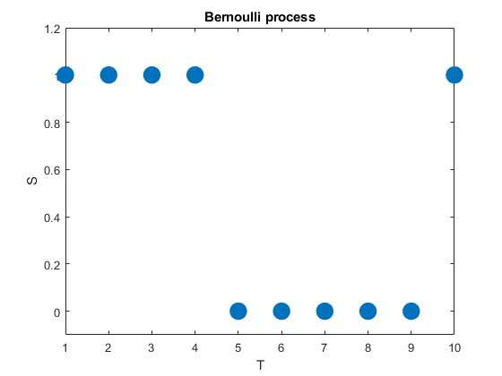
A very simple stochastic process is the Bernoulli process, which is a sequence of independent and identically distributed (iid) random variables. The value of each random variable can be one of two values, typically \(0\) and \(1\), but they could be also \(-1\) and \(+1\) or \(H\) and \(T\). To generate this stochastic process, each random variable takes one value, say, \(1\) with probability \(p\) or the other value, say, \(0\) with probability \(1-p\).
We can can liken this stochastic process to flipping a coin, where the probability of a head is \(p\) and its value is \(1\), while the value of a tail is \(0\). In other words, a Bernoulli process is a sequence of iid Bernoulli random variables. The Bernoulli process has the counting numbers (that is, the positive integers) as its index set, meaning \(T=1,\dots\), while in this example the state space is simply \(S=\{0,1\}\).
(We can easily generalize the Bernoulli process by having a sequence of iid variables with the same probability space.)
Random walks
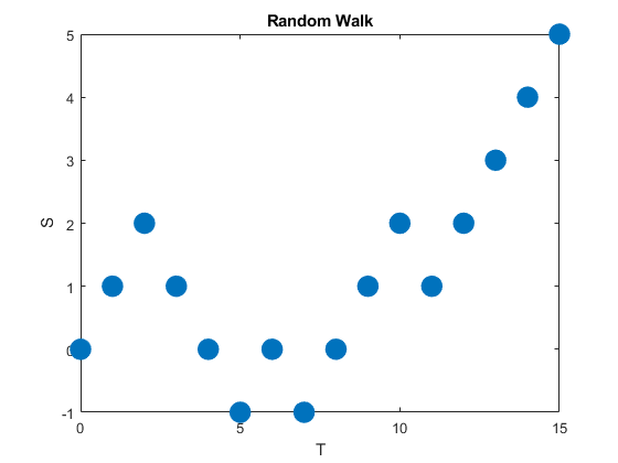
A random walk is a type of stochastic process that is usually defined as sum of a sequence of iid random variables or random vectors in Euclidean space. Given random walks are formed from a sum, they are stochastic processes that evolve in discrete time. (But some also use the term to refer to stochastic processes that change in continuous time.)
A classic example of this stochastic process is the simple random walk, which is based on a Bernoulli process, where each iid Bernoulli variable takes either the value positive one or negative one. More specifically, the simple random walk increases by one with probability, say, \(p\), or decreases by one with probability \(1-p\). The index set of this stochastic process is the natural numbers, while its state space is the integers.
Random walks can be defined in more general settings such as \(n\)- dimensional Euclidean space. There are other types of random walks, defined on different mathematical objects, such as lattices and groups, and in general they are highly studied and have many applications in different disciplines.
Markov processes
One important way for classifying stochastic processes is the stochastic dependence between random variables. For the Bernoulli process, there was no dependence between any random variable, giving a very simple stochastic process. But this is not a very interesting stochastic process.
A more interesting (and typically useful) stochastic process is one in which the random variables depend on each other in some way. For example, the next position of a random walk depends on the current position, which in turn depends on the previous position.
A large family of stochastic processes in which the next value depends on the current value are called Markov processes or Markov chains. (Both names are used. The term Markov chain is largely used when either the state space or index is discrete, but there does not seem to be an agreed upon convention. When I think Markov chain, I think discrete time.) The definition of a Markov process has a property that constrains the dependence between the random variables, as the next random variable only depends on the current random variable, and not all the previous random variables. This constraint on the dependence typically renders Markov processes more tractable than general stochastic processes.
It would be difficult to overstate the importance of Markov processes. Their study and application appear throughout probability, science, and technology.
Counting processes
A counting process is a stochastic process that takes the values of non-negative integers, meaning its state space is the counting numbers, and is non-decreasing. A simple example of a counting process is an asymmetric random walk, which increases by one with some probability \(p\) or remains the same value with probability \(1-p\). In other words, the accumulative sum of a Bernoulli process. This is an example of a discrete-time counting process, but continuous-time ones also exist.
A counting process can be also interpreted as a counting as a random counting measure on the index set.
Two important stochastic processes
The most two important stochastic processes are the Poisson process and the Wiener process (often called Brownian motion process or just Brownian motion). They are important for both applications and theoretical reasons, playing fundamental roles in the theory of stochastic processes. In future posts I’ll cover both the Wiener process and the Poisson process.
Code
The code used to create the plots in this post is found here on my code repository. The code exists in both MATLAB and Python.
Further reading
There are many, many books covering the fundamentals of modern probability theory, including those (in roughly increasing order of difficulty) by Grimmett and Stirzaker, Karr, Rosenthal, Shiryaev, Durrett, and Billingsley. A very quick introduction is given in this web article.
The development of stochastic processes is one of the great achievements in modern mathematics. Researchers and practitioners have both studied them in great depth and found many applications for them. Consequently, there is no shortage of literature on stochastic processes. For example:
- Grimmett and Stirzaker, Probability and Random Processes;
- Ross, Stochastic Processes;
- Karlin and Taylor, A First Course in Stochastic Processes;
- Karlin and Taylor, A Second Course in Stochastic Processes;
- Rogers and Williams, Diffusions, Markov Processes, and Martingales: Volume 1;
- Resnick, Adventures in Stochastic Processes;
- Parzen, Stochastic Processes;
- Durrett, Essentials of Stochastic Processes;
- Rosenthal, A First Look at Stochastic Processes.
Finally, one of the main pioneers of stochastic processes was Joseph Doob. His seminal book was simply called Stochastic Processes.