Binomial point process

The binomial point process is arguably the simplest point process. It consists of a non-random number of points scattered randomly and independently over some bounded region of space. In this post I will describe the binomial point process, how it leads to the Poisson point process, and its historical role as stars in the sky.

The binomial point process is an important stepping stone in the theory of point process. But I stress that for mathematical models, I would always use a Poisson point process instead of a binomial one. The only exception would be if you were developing a model for a small, non-random number of points.

Uniform binomial point process

We start with the simplest binomial point process, which has uniformly located points. (I described simulating this point process in an early post. The code is here.)

Definition

Consider some bounded (or more precisely, compact) region, say, \(W\), of the plane plane \(\mathbb{R}^2\), but the space can be more general.  The uniform binomial point process is created by scattering \(n\) points uniformly and independently across the set \(W\).
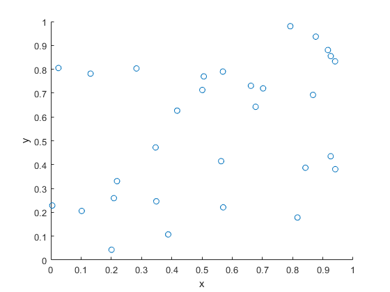
A single realization of a binomial point process with n=30 points. The points are uniformly and independently scattered across a unit square.

Distribution

Consider a single point uniformly scattered in the region \(W\), giving a binomial point process with \(n=1\).  We look at some region \(B\), which is a subset of \(W\), implying \(B\subseteq W\).  What is the probability that the single point \(X\) falls in region \(B\)?

First we write \(\nu(W)\) and \(\nu(B)\)  to denote the respective areas (or more precisely, Lebesgue measures) of the regions \(W\) and \(B\), hence \(\nu(B)\leq \nu(W)\). Then this probability, say, \(p\), is simply the ratio of the two areas, giving

$$p= P(X\in B)=\frac{\nu(B)}{\nu(W)}.$$

The event of a single point being found in the set \(B\) is a single Bernoulli trial, like flipping a single coin. But if there are \(n\) points, then there are \(n\) Bernoulli trials, which bring us to the binomial distribution.

For a uniform binomial point process \(N_W\), the number of randomly located points being found in a region \(B\) is a binomial random variable, say, \(N_W(B)\), with probability parameter \(p=\nu(B)/ \nu(W)\). The probability mass function of \(N_W(B)\) is

$$ P(N_W(B)=k)={n\choose k} p^k(1-p)^{n-k}. $$

We can write the expression more explicitly

$$ P(N_W(B)=k)={n\choose k} \left[\frac{\nu(B)}{ \nu(W)}\right]^k\left[1-\frac{\nu(B)}{\nu(W)}\right]^{n-k}. $$

Poisson limit

Poisson random variable

A standard exercise in introductory probability is deriving the Poisson distribution by taking the limit of the binomial distribution. This is done by sending \(n\) (the total number of Bernoulli trials) to infinity while keeping the binomial mean \(\mu:=p n\) fixed, which sends the probability \(p=\mu/n\) to zero.

More precisely, for \(\mu\geq0\), setting \(p_n=\mu/n \) and keeping \(\mu :=p_n n\) fixed, we have the limit result

$$\lim_{n\to \infty} {n \choose k} p_n^k (1-p_n)^{n-k} = \frac{\mu^k}{k!}\, e^{-\mu}.$$

We can use, for example, Stirling’s approximation to prove this limit result.

We can make the same limit argument with the binomial point process.

Homogeneous Poisson point process

We consider the intensity of the uniform binomial point process, which is the average number of points in a unit area. For a binomial point process, this is simply

$$\lambda := \frac{n}{\nu(W)}.$$

For the Poisson limit, we expand the region \(W\) so it covers the whole plane \(\mathbb{R}^2\), while keeping the intensity \(\lambda = n/\nu(W)\) fixed. This means that the area \(\nu(W)\) approaches infinity while the probability \(p=\nu(B)/\nu(W)\) goes to zero. Then in the limit we arrive at the homogeneous Poisson point process \(N\) with intensity \(\lambda\).

The number of points of \(N\) falling in the set \(B\) is a random variable \(N(B)\) with the probability mass function

$$ P(N(B)=k)=\frac{[\lambda \nu(B)]^k}{k!}\,e^{-\lambda \nu(B)}. $$

General binomial point process

Typically in point process literature, one first encounters the uniform binomial point process. But we can generalize it so the points are distributed according to some general distribution.

Definition

We write \(\Lambda\) to denote a non-negative Radon measure on \(W\), meaning \(\Lambda(W)< \infty\) and \(\Lambda(B)\geq 0\) for all (measurable) sets \(B\subseteq W\).  We can also assume a more general space for the underlying space such as a compact metric space, which is (Borel) measurable. But the intuition still works for compact region of the plane \(\mathbb{R}^2\).

For the \(n\) points, we assume each point is distributed according to the probability measure

$$\bar{\Lambda}= \frac{\Lambda}{\Lambda(W)}.$$

The resulting point process is a general binomial point process. The proofs for this point process remain essentially the same, replacing the Lebesgue measure \(\nu\), such as area or volume, with the non-negative measure \(\Lambda\).

Example

A typical example of the intensity measure \(\Lambda\) has the form

$$\Lambda(B)= \int_B f(x) dx\,,$$

where \(f\) is a non-negative density function on \(W\). Then the probability density of a single point is

$$ p(x) = \frac{1}{c}f(x),$$

where \(c\) is a normalization constant

$$c= \int_W f(x) dx\,.$$

On a set \(W \subseteq \mathbb{R}^2\) using Cartesian coordinates, a specific example of the density \(f\) is

$$ f(x_1,x_2) = \lambda e^{-(x_1^2+x_2^2)}.$$

Distribution

Assuming a general binomial point process \(N_W\) on \(W\), we can use the previous arguments to obtain the binomial distribution

$$ P(N_W(B)=k)={n\choose k} \left[\frac{\Lambda(B)}{\Lambda(W)}\right]^k\left[1-\frac{\Lambda(B)}{\Lambda(W)}\right]^{n-k}. $$

General Poisson point process

We can easily adapt the Poisson limit arguments for the general binomial Poisson point process, which results in the general Poisson point process \(N\) with intensity measure \(\Lambda\). The number of points of \(N\) falling in the set \(B\) is a random variable \(N(B)\) with the probability mass function

$$ P(N(B)=k)=\frac{[\Lambda(B)]^k}{k!}\, e^{-\Lambda(B)}. $$

History: Stars in the sky

The uniform binomial point process is an example of a spatial point process. With points being scattered uniformly and independently, its sheer simplicity makes it a natural choice for an early spatial model. But which scattered objects?

Perhaps not surprisingly, it is trying to understand star locations where we find the earliest known example of somebody describing something like a random point process. In 1767 in England John Michell wrote:

what it is probable would have been the least apparent distance of any two or more stars, any where in the whole heavens, upon the supposition that they had been scattered by mere chance, as it might happen

As an example, Michelle studied the six brightest stars in the Pleiades star cluster. He concluded the stars were not scattered by mere chance. Of course “scattered by mere chance” is not very precise in today’s probability language, but we can make the reasonable assumption that Michell meant the points were uniformly and independently scattered.

Years later in 1860 Simon Newcomb  examined Michell’s problem, motivating him to derive the Poisson distribution as the limit of the binomial distribution. Newcomb also studied star locations. Stephen Stigler considers this as the first example of applying the Poisson distribution to real data, pre-dating the famous work by Ladislaus Bortkiewicz who studied rare events such as deaths from horse kicks. We also owe Bortkiewicz the terms Poisson distribution and stochastic (in the sense of random).

Code

Here, on my repository, are some pieces of code that simulate a uniform binomial point process on a rectangle.

Further reading

For an introduction to spatial statistics, I suggest the lectures notes by Baddeley, which form Chapter 1 of these published lectures, edited by Baddeley, Bárány, Schneider, and Weil. The binomial point process is covered in Section 1.3.

The binomial point process is also covered briefly in the classic text Stochastic Geometry and its Applications by Chiu, Stoyan, Kendall and Mecke; see Section 2.2. Similar material is covered in the book’s previous edition by Stoyan, Kendall and Mecke.

Haenggi also wrote a readable introductory book called Stochastic Geometry for Wireless networks, where he gives the basics of point process theory. The binomial point process is covered in Section 2.4.4.

For some history on point processes and the Poisson distribution, I suggest starting with the respective papers:

  • Guttorp and Thorarinsdottir, What Happened to Discrete Chaos, the Quenouille Process, and the Sharp Markov Property?;
  • Stigler, Poisson on the Poisson distribution.

Histories of the Poisson distribution and the Poisson point process are found in the books:

Summary: Poisson simulations

Here’s a lazy summary post where I list all the posts on various Poisson simulations. I’ve also linked to code, which is found on this online repository. The code is typically written in MATLAB and Python.

Posts

Poisson point processes

Some simulations of Poisson point processes are also covered in this post on the Julia programming language:

Checking simulations

Poisson line process

Poisson random variables

Voronoi tessellations in architecture

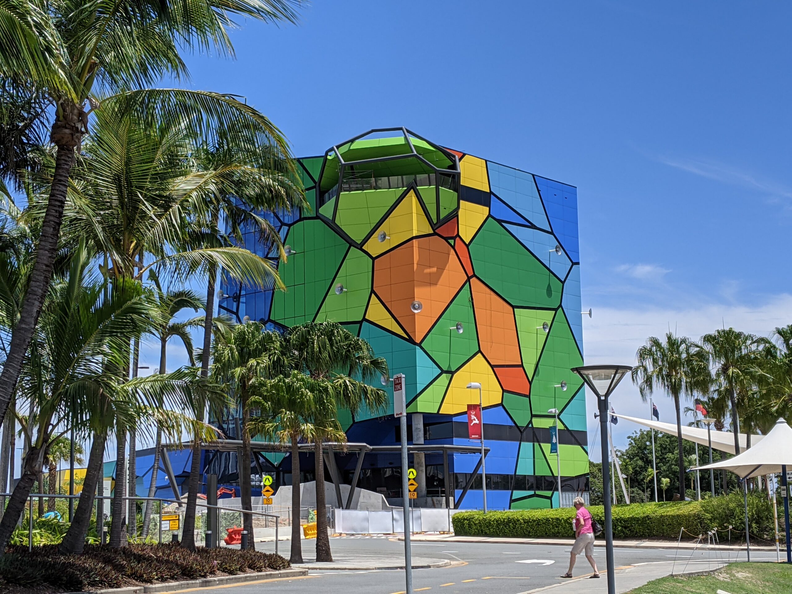
A colleague just sent me this photo of a colourful building on the Gold Coast. The building is the new Home of the Arts (HOTA) Gallery, as detailed here. It is covered in a Voronoi tessellation. I described this very useful geometrical object in a previous post.

The New HOTA Gallery with a Voronoi tessellation on the outside.

A casual Google reveals that other buildings have Voronoi-inspired architecture. For example, The Fry building at the University of Bristol in Britain, which fittingly houses the mathematics department.

The Fry Building at the University of Bristol (Source)

The building for the Alibaba headquarters in China also evokes Voronoi imagery. But those Voronoi constructions do no feature the colours of the HOTA Gallery, which is reminiscent of diagrams produced by scientific plotting packages.

(Of course I don’t mind the odd Voronoi tesselation. For example, a couple of months ago I set for my website image a Voronoi tesselation, created by the Franco-German artist Plaisance Puisatier. And the cover of a book I co-wrote has a diagram based on the signal-to-interference ratio, which can be considered as a generalization of a Voronoi tessellation.)

Mathematical buildings

Another building that employs an interesting geometrical object is RMIT’s Storey Hall, located in Melbourne. It features Penrose tiling, which is an example of a non-periodic tiling. Loosely speaking, that means if you tile an infinite plane with a given a set of tiles, then no translation of the plane will yield the same pattern again. The Penrose tiling is also inside the building, as you can see on this website.

On topic of non-periodic tiling, the buildings at Federation Square in Melbourne are covered by pinwheel tiling, as shown on this mathematics website, which is also non-periodic. According to Wikipedia, Charles Radin proposed this tiling based on a construction by the late and famous John Conway who died earlier this year, being yet another victim of the pandemic.

Mathematical architects

While writing this post, I noticed that both the HOTA Gallery and Storey Hall were designed by ARM Architecture. Some of their other buildings have a geometrical aspect. Clearly they have a mathematical inclination.

Simulating Poisson random variables in Fortran

The hint’s in the title. I wrote a simple function in Fortran for simulating (or sampling) Poisson random variables. (More precisely, I should say that the function generates Poisson variates.) I used the simple direct method. This method is based on the exponential inter-arrival times of the Poisson (stochastic) process.

My code should not be used for large Poisson parameter values (larger than, say, 20 or 30), as the code may be too slow. Other methods exist for larger parameter values, which I’ve discussed previously.

I just use the standard Fortran function random_number for generating (pseudo-)random numbers. I am not an expert in Fortran, but my Poisson function seems to work fine. I wrote and ran a simple test that estimates the first and second moments, which should match for Poisson variables.

My Fortran code is very similar to the code that I wrote in C and C#, which is located here. You should be able to run it on this website or similar ones that can compile Fortran (95) code.

Further reading

For various Poisson simulation methods, see the stochastic simulation books by Devroye (Section X.3) or Fishman (Section 8.16). There’s a free online version of Devroye’s book here. The book by Gentle (Section 5.2.8) also briefly covers Poisson variables.

In this post on generating Poisson variates, John D. Cook briefly discusses the direct method (for small Poisson parameter values), as well as a rejection method from a 1979 paper by Atkinson.

I wrote the Poisson code using Fortran 95. There are various books and websites on Fortran. The website tutorialspoint.com gives a good introduction to Fortran. You can also edit, compile and run your Fortran code there with its online Fortran editor. I found this short summary a good start. For alternative Fortran code of a Poisson generator, consult the classic book Numerical Recipes, though I believe the book versions only exist for Fortran 77 and Fortran 90.

Code

On this page I’ve only included the code of the functions for generating uniform and Poisson variates. The rest of the code, including the test, is located here.

!Poisson function -- returns a single Poisson random variable
function funPoissonSingle(lambda) result(randPoisson)
real, intent(in) :: lambda !input
real :: exp_lambda !constant for terminating loop
real :: randUni !uniform variable
real :: prodUni !product of uniform variables
integer :: randPoisson !Poisson variable

exp_lambda= exp(-lambda) 

!initialize variables
randPoisson = -1;
prodUni = 1;
do while (prodUni > exp_lambda)
   randUni = funUniformSingle() !generate uniform variable
   prodUni = prodUni * randUni; !update product
   randPoisson = randPoisson + 1 !increase Poisson variable
end do
end function

!Uniform function -- returns a standard uniform random variable
function funUniformSingle() result(randUni)
real randUni;
call random_seed
call random_number(randUni)

end function

Frozen code

My simulation code has been frozen and buried in Norway. Well, some of my code that I keep on a GitHub repository has become part of a code preservation project. Consequently, beneath my profile it reads:

Arctic Code Vault Contributor

This is part of what is called the GitHub Archive Program. The people behind it aim to preserve large amounts of (open source) code for future generations in thousands and thousands of years time. But how do they do that?

Well, basically, the good people at GitHub chose and converted many, many, many lines of code into certain error-resistant formats, such as QR code. They then printed it all out and buried it deep in an abandoned mine shaft in frozen Norway. (The frozen and stable Norway is also home to a famous seed bank.)

My code in this project includes most of the code that has appeared in these posts. Of course my contribution is just a drop in the vast code ocean of this project. In fact, at least two or three of my colleagues have also had their code put into deep freeze.

Still, it’s a nice thought to know that stuff I wrote, including code for these very posts, will be potentially around for a very long time.

Simulating a Poisson point process on a n-dimensional sphere

In the previous post I outlined how to simulate or sample a homogeneous Poisson point process on the surface of a sphere. Now I will consider a homogeneous Poisson point process on the \((n-1)-\) sphere, which is the surface of the Euclidean ball in \(n\) dimensions.

This is a short post because it immediately builds off the previous post. For positioning the points uniformly, I will use Method 2 from that post, which uses normal random variables, as it immediately gives a fast method in \(n\) dimensions.

I wrote this post and the code more for curiosity than any immediate application. But simulating a Poisson point process in this setting requires placing points uniformly on a sphere. And there are applications in that, such as Monte Carlo integration methods, as mentioned in this post, which nicely details different sampling methods.

Steps

As is the case for other shapes, simulating a Poisson point process requires two steps.

Number of points

The number of points of a Poisson point process on the surface of a sphere of radius \(r>0\) is a Poisson random variable. The mean of this random variable is \(\lambda S_{n-1}\), where \(S_{n-1}\) is the surface area of the sphere.  For a ball embedded in \(n\) dimension, the area of the corresponding sphere is given by

$$S_{n-1} = \frac{2 \pi ^{n/2}  }{\Gamma(n/2)} r^{n-1},$$

where \(\Gamma\) is the gamma function, which is a natural generalization of the factorial. In MATLAB, we can simply use the function gamma.  In Python, we need to use the SciPy function scipy.special. gamma.

Locations of points

For each point on the sphere, we generate \(n\) standard normal or Gaussian random variables, say, \(W_1, \dots, W_n\), which are independent of each other. These random variables are the Cartesian components of the random point. We rescale the components by the Euclidean norm, then multiply by the radius \(r\).

For \(i=1,\dots, n\), we obtain

$$X_i=\frac{rW_i}{(W_1^2+\cdots+W_n^2)^{1/2}}.$$

These are the Cartesian coordinates of a point uniformly scattered on a  sphere with radius \(r\) and a centre at the origin.

How does it work?

In the post on the circle setting, I gave a more detailed outline of the proof, where I said the method is like the Box-Muller transform in reverse. The joint density of the normal random variables is from a multivariate normal distribution with zero correlation. This joint density a function of the Cartesian equation for a sphere. This means the density is constant on the sphere, implying that the angle of the point \((W_1,\dots, W_n)\) will be uniformly distributed.

The vector formed from the normal variables \((W_1,\dots,W_n)\) is a random variable with a chi distribution.  But the final vector, which stretches from the origin to the point \((X_1,\dots,X_n)\), has length one, because we rescaled it with the Euclidean norm.

Code

The code for all my posts is located online here. For this post, the code in MATLAB and Python is here.

Further reading

I recommend this blog post, which discusses different methods for randomly placing points on spheres and inside spheres (or, rather, balls) in a uniform manner.  (Embedded in two dimensions, a sphere is a circle and a ball is a disk.)

Our Method 2 for positioning points uniformly, which uses normal variables, comes from the paper:

  • 1959, Muller, A note on a method for generating points uniformly on n-dimensional spheres.

Two recent works on this approach are the papers:

  • 2010, Harman and Lacko, On decompositional algorithms for uniform sampling from -spheres and -balls;
  • 2017, Voelker, Gosman, Stewart, Efficiently sampling vectors and coordinates.

Simulating a Poisson point process on a sphere

In this post I’ll describe how to simulate or sample a homogeneous Poisson point process on the surface of a sphere. I have already simulated this point process on a rectangle, triangle disk, and circle.

Of course, by sphere, I mean the everyday object that is the surface of a three-dimensional ball, where this two-dimensional object is often denoted by \(S^2\).  Mathematically, this is a generalization from a Poisson point process on a circle, which is slightly simpler than randomly positioning points on a disk.  I recommend reading those two posts first, as a lot of the material presented here builds off them.

I have not needed such a simulation in my own work, but I imagine there are many reasons why you would want to simulate a Poisson point process on a sphere. As some motivation, we can imagine these points on a sphere representing, say, meteorites or lightning hitting the Earth.

The generating the number of points is not difficult. The trick is positioning the points on the sphere in a uniform way.  As is often the case, there are various ways to do this, and I recommend this post, which lists the main ones.  I will use two methods that I consider the most natural and intuitive ones, namely using spherical coordinates and normal random variables, which is what I did in the post on the circle.

Incidentally, a simple modification allows you to scatter the points uniformly inside the sphere, but you would typically say ball in mathematics, giving a Poisson point process inside a ball; see below for details.

Steps

As always, simulating a Poisson point process requires two steps.

Number of points

The number of points of a Poisson point process on the surface of a sphere of radius \(r>0\) is a Poisson random variable with mean \(\lambda S_2\), where \(S_2=4\pi r^2\) is the surface area of the sphere. (In this post I give some details for simulating or sampling Poisson random variables or, more accurately, variates.)

Locations of points

For any homogeneous Poisson point process, we need to position the points uniformly on the underlying space, which is in this case is the sphere. I will outline two different methods for positioning the points randomly and uniformly on a sphere.

Method 1: Spherical coordinates

The first method is based on spherical coordinates \((\rho, \theta,\phi)\), where the radial coordinate \(\rho\geq 0\), and the angular coordinates \(0 \leq \theta\leq 2\pi\) and \(0\leq \phi \leq \pi\). The change of coordinates gives \(x=\rho\sin(\theta)\cos(\phi)\), \(y=\rho\sin(\theta)\sin(\phi)\), and \(z=\rho\cos(\phi)\).

Now we use Proposition 1.1 in this paper. For each point, we generate two uniform variables \(V\) and \(\Theta\) on the respective intervals \((-1,1)\) and \((0,2\pi)\). Then we place the point with the Cartesian coordinates

$$X =  r  \sqrt{1-V^2} \cos\Theta, $$

$$Y =  r  \sqrt{1-V^2}\sin\Theta, $$

$$ Z=r V. $$

This method places a uniform point on a sphere with a radius \(r\).

How does it work?

I’ll skip the precise details, but give some interpretation of this method. The random variable \(\Phi := \arccos V\) is the \(\phi\)-coordinate of the uniform point, which implies \(\sin \Phi=\sqrt{1-V^2}\), due to basic trigonometric identities.  The area element in polar coordinates is \(dA = \rho^2 \sin\phi d\phi d\theta \), which is constant with respect to \(\theta\). After integrating with respect to \(\phi\),  we see that the random variable \(V=\cos\Phi\) needs to be uniform (instead of \(\Phi\)) to ensure the point is uniformly located on the surface.

Method 2: Normal random variables

For each point, we generate three standard normal or Gaussian random variables, say, \(W_x\), \(W_y\), and \(W_z\), which are independent of each other. (The term standard here means the normal random variables have mean \(\mu =0\) and standard deviation \(\sigma=1\).)  The three random variables are the Cartesian components of the random point. We rescale the components by the Euclidean norm, then multiply by the radius \(r\), giving

$$X=\frac{rW_x}{(W_x^2+W_y^2+W_z^2)^{1/2}},$$

$$Y=\frac{rW_y}{(W_x^2+W_y^2+W_z^2)^{1/2}},$$

$$Z=\frac{rW_z}{(W_x^2+W_y^2+W_z^2)^{1/2}}.$$

These are the Cartesian coordinates of a point uniformly scattered on a  sphere with radius \(r\) and a centre at the origin.

How does it work?

The procedure is somewhat like the Box-Muller transform in reverse. In the post on the circle setting,  I gave an outline of the proof, which I recommend reading. The joint density of the normal random variables is from a multivariate normal distribution with zero correlation. This joint density is constant on the sphere, implying that the angle of the point \((W_x, W_y, W_z)\) will be uniformly distributed.

The vector formed from the normal variables \((W_x, W_y,W_z)\) is a random variable with a chi distribution.  We can see that the vector from the origin to the point \((X,Y,Z)\) has length one, because we rescaled it with the Euclidean norm.

Plotting

Depending on your plotting software, the points may more resemble points on an ellipsoid than a sphere due to the different scaling of the x, y and z axes. To fix this in MATLAB, run the command: axis square. In Python, it’s not straightforward to do this, as it seems to lack an automatic function, so I have skipped it.

Results

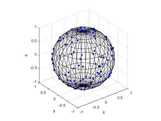
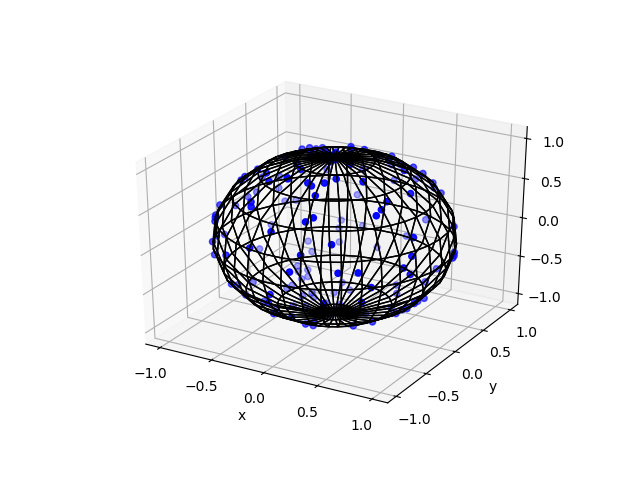
I have presented some results produced by code written in MATLAB and Python. The blue points are the Poisson points on the sphere. I have used a surface plot (with clear faces) to illustrate the underling sphere in black.

MATLAB

Python

Note: The aspect ratio in 3-D Python plots tends to squash the sphere slightly, but it is a sphere.

Code

The code for all my posts is located online here. For this post, the code in MATLAB and Python is here.  In Python I used the library mpl_toolkits for doing 3-D plots.

Poisson point process inside the sphere

Perhaps you want to simulate a Poisson point process inside the ball.  There are different ways we can do this, but I will describe just one way, which builds off Method 1 for positioning the points uniformly. (In a later post, I will modify Method 2, giving a way to uniformly position points inside the ball.)

For this simulation method, you need to make two simple modifications to the simulation procedure.

Number of points

The number of points of a Poisson point process inside a sphere of radius \(r>0\) is a Poisson random variable with mean \(\lambda V_3\), where \(V_3=4\pi r^3\) is the volume of the sphere.

Locations of points

We will modify Method 1 as outlined above. To sample the points uniformly in the sphere, you need to generate uniform variables on the unit interval \((0,1)\), take their cubic roots, and then, multiply them by the radius \(r\). (This is akin to the step of taking the square root in the disk setting.) The random variables for the angular coordinates are generated as before.

Further reading

I recommend this blog post, which discusses different methods for randomly placing points on spheres and inside spheres (or, rather, balls) in a uniform manner.  (Embedded in two dimensions, a sphere is a circle and a ball is a disk.)

Our Method 2 for positioning points uniformly, which uses normal variables, comes from the paper:

  • 1959, Muller, A note on a method for generating points uniformly on n-dimensional spheres.

This sampling method relies upon old observations that normal variables are connected to spheres and circles. I also found this post on a similar topic. Perhaps not surprisingly, the above paper is written by the same Muller behind the Box-Muller method for sampling normal random variables.

Update: The connection between the normal distribution and rotational symmetry has been the subject of some recent 3Blue1Brown videos on YouTube.

Here is some sample Python code for creating a 3-D scatter plot.

Simulating a Poisson point process on a circle

In this post, I’ll take a break from the more theoretical posts. Instead I’ll describe how to simulate or sample a homogeneous Poisson point process on a circle.  I have already simulated this point process on a rectangle, triangle and disk. In some sense, I should have done this simulation method before the disk one, as it’s easier to simulate. I recommend reading that post first, as the material presented here builds off it.

Sampling a homogeneous Poisson point process on a circle is rather straightforward.  It just requires using a fixed radius and uniformly choose angles from interval \((0, 2\pi)\). But the circle setting gives an opportunity to employ a different method for positioning points uniformly on circles and, more generally, spheres. This approach uses Gaussian random variables, and it becomes much more efficient when the points are placed on high dimensional spheres.

Steps

Simulating a Poisson point process requires two steps: simulating the random number of points and then randomly positioning each point.

Number of points

The number of points of a Poisson point process on circle of radius \(r>0\) is a Poisson random variable with mean \(\lambda C\), where \(C=2\pi r\) is the circumference of the circle.  You just need to be able to need to produce (pseudo-)random numbers according to a Poisson distribution.

To generate Poisson variables in MATLAB,  use the poissrnd function with the argument \(\lambda C\).  In Python, use either the scipy.stats.poisson or numpy.random.poisson function from the SciPy or NumPy libraries. (If you’re curious how Poisson simulation works, I suggest seeing this post for details on sampling Poisson random variables or, more accurately, variates.)

Locations of points

For a homogeneous Poisson point process, we need to uniformly position points on the underlying space, which is this case is a circle. We will look at two different ways to position points uniformly on a circle. The first is arguably the most natural approach.

Method 1: Polar coordinates

We use polar coordinates due to the nature of the problem. To position all the points uniformly on a circle, we simple generate uniform numbers on the unit interval \((0,1)\). We then multiply these random numbers by \(2\pi\).

We have generated polar coordinates for points uniformly located on the circle. To plot the points, we have to convert the coordinates back to Cartesian form by using the change of coordinates:  \(x=\rho\cos(\theta)\) and \(y=\rho\sin(\theta)\).

Method 2: Normal random variables

For each point, we generate two standard normal or Gaussian random variables, say, \(W_x\) and \(W_y\), which are independent of each other. (The term standard here means the normal random variables have mean \(\mu =0\) and standard deviation \(\sigma=1\).) These two random variables are the Cartesian components of a random point.  We then rescale the two values by the Euclidean norm, giving

$$X=\frac{W_x}{(W_x^2+W_y^2)^{1/2}},$$

$$Y=\frac{W_y}{(W_x^2+W_y^2)^{1/2}}.$$

These are the Cartesian coordinates of points uniformly scattered around a unit circle with centre at the origin. We multiply the two random values \(X\) and \(Y\) by the \(r>0\)  for a circle with radius \(r\).

How does it work?

The procedure is somewhat like the Box-Muller transform in reverse. I’ll give an outline of the proof. The joint density of the random variables \(W_x\) and \(W_y\) is that of the bivariate normal distribution with zero correlation, meaning it has the joint density

$$ f(x,y)=\frac{1}{2\pi}e^{[-(x^2+y^2)/2]}.$$

We see that the function \(f\) is a constant when we trace around any line for which \((x^2+y^2)\) is a constant, which is simply the Cartesian equation for a circle (where the radius is the square root of the aforementioned constant). This means that the angle of the point \((W_x, W_y)\) will be uniformly distributed.

Now we just need to look at the distance of the random point. The vector formed from the pair of normal variables \((W_x, W_y)\) is a Rayleigh random variable.  We can see that the vector from the origin to the point \((X,Y)\) has length one, because we rescaled it with the Euclidean norm.

Results

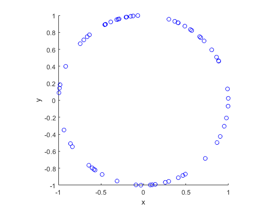
I have presented some results produced by code written in MATLAB and Python. The blue points are the Poisson points on the sphere. I have used a surface plot (with clear faces) in black to illustrate the underling sphere.

MATLAB

Python

Code

The code for all my posts is located online here. For this post, the code in MATLAB and Python is here.

Further reading

I recommend this blog post, which discusses different methods for randomly placing points on spheres and inside spheres (or, rather, balls) in a uniform manner.  (Embedded in two dimensions, a sphere is a circle and a ball is a disk.) A key paper on using normal variables is the following:

  • 1959, Muller, A note on a method for generating points uniformly on n-dimensional spheres.

As I mentioned in the post on the disk, the third edition of the classic book Stochastic Geometry and its Applications by Chiu, Stoyan, Kendall and Mecke details on page 54 how to uniformly place points on a disk.  It just requires a small modification for the circle.

Coverage probability in wireless networks with determinantal scheduling

My collaborators and I uploaded a manuscript:

  • Błaszczyszyn, Brochard, and Keeler, Coverage probability in wireless networks with determinantal scheduling.

https://arxiv.org/abs/2006.05038

Details

The paper builds off some previous work by us that uses a (relatively) new model in machine learning:

  • Błaszczyszyn and Keeler, Determinantal thinning of point processes with network learning applications.

https://arxiv.org/abs/1810.08672

The new machine learning model is based on a special type of point process called a determinantal point process. It was originally called a Fermion point process. These are useful point processes as the exhibit certain closure properties under certain operations such independent thinning.

Kulesza and Taskar introduced and developed the framework for using determinantal point processes for machine learning models.

Code

The MATLAB code for the producing the results in the paper can be found here:

https://github.com/hpaulkeeler/detcov_matlab

I also re-wrote the MATLAB code into Python:

https://github.com/hpaulkeeler/detcov_python

Cox point process

In previous posts I have often stressed the importance of the Poisson point process as a mathematical model. But it can be unsuitable for certain mathematical models.  We can generalize it by first considering a non-negative random measure, called a driving or directing measure. Then a Poisson point process, which is independent of the random driving measure, is generated by using the random measure as its intensity or mean measure. This doubly stochastic construction gives what is called a Cox point process.

In practice we don’t typically observe the driving measure. This means that it’s impossible to distinguish a Cox point process from a Poisson point process if there’s only one realization available. By conditioning on the random driving measure, we can use the properties of the Poisson point process to derive those of the resulting Cox point process.

By the way, Cox point processes are also known as doubly stochastic Poisson point processes. Guttorp and Thorarinsdottir argue that we should call them the Quenouille point processes, as Maurice Quenouille introduced an example of it before Sir David Cox. But I opt for the more common name.

In this post I’ll cover a couple examples of Cox point processes. But first I will need to give a more precise mathematical definition.

Definition

We consider a point process defined on some underlying mathematical space \(\mathbb{S}\), which is sometimes called the carrier space or state space.  The underlying space is often the real line \(\mathbb{R}\), the plane \(\mathbb{R}^2\), or some other familiar mathematical space like a square lattice.

For the first definition, we use the concept of a random measure.

Let \(M\) be a non-negative random measure on \(\mathbb{S} \). Then a point process \(\Phi\) defined on some underlying space \(\mathbb{S}\) is a Cox point process driven by the intensity measure \(M\) if the conditional distribution of \(\Phi\) is a Poisson point process with intensity function \(M\).

We can give a slightly less general definition of a Cox  point process by using a random intensity function.

Let \(Z=\{Z(x):x\in\mathbb{S} \}\) be a non-negative random field such that with probability one, \(x\rightarrow Z(x)\) is a locally integrable function. Then a point process \(\Phi\) defined on some underlying space \(\mathbb{S}\) is a Cox point process driven by \(Z\) if the conditional distribution of \(\Phi\) is a Poisson point process with intensity function \(Z\).

The random driving measure \(M\) is then simply the integral
$$
M(B)=\int_B Z(x)\, dx , \quad B\subseteq S.
$$

Over-dispersion

The random driving measures take different forms, giving different Cox point processes. But there is a general observation that can be made for all Cox point processes. For any region \(B \subseteq S\), it can be shown that the number of points \(\Phi (B)\) adheres to the inequality
$$
\mathbb{Var} [\Phi (B)] \geq \mathbb{E} [\Phi (B)],
$$

where \(\mathbb{Var} [\Phi (B)] \) is the variance of the random variable \(\Phi (B)\).  As a comparison, for a Poisson point process \(\Phi’\), the variance of \(\Phi’ (B)\) is simply \(\mathbb{Var} [\Phi’ (B)] =\mathbb{E} [\Phi’ (B)]\).  Due to its greater variance, the Cox point process is said to be over-dispersed compared to the Poisson point process.

Special cases

There is an virtually unlimited number of ways to define a random driving measure, where each one yields a different a Cox point process. But in general we are restricted by examining only tractable and interesting Cox point processes. I will give some common examples, but I stress that the Cox point process family is very large.

Mixed Poisson point process

For the random driving measure \(M\), an obvious example is the product form \(M= Y \mu \), where \(Y\) is some independent non-negative random variable and \(\mu\) is the Lebesgue measure on \(\mathbb{S}\). This driving measure gives the mixed Poisson point process. The random variable \(Y\) is the only source of randomness.

Log-Gaussian Cox point process

Instead of a random variable, we can use a non-negative random field to define a random driving measure.  We then have the product \(M= Y \mu \), where \(Y\) is now some independent non-negative random field. (A random field is a collection of random variables indexed by some set, which in this case is the underlying space \(\mathbb{S}\).)

Arguably the most tractable and used random field is the Gaussian random field. This random field, like Gaussian or normal random variables, takes both negative and positive values. But if we define the random field such that its logarithm is a Gaussian field \(Z\), then we obtain the non-negative random driving measure \(M=\mu e^Z \), giving the log-Gaussian Cox point process.

This point process has found applications in spatial statistics.

Cox-Poisson line-point process

To construct this Cox point process, we first consider a Poisson line process, which I discussed previously.  Given a Poisson line process, we then place an independent one-dimensional Poisson point process on each line. We then obtain an example of a Cox point process, which we could call a Cox line-point process orCox-Poisson line-point process. (But I am not sure of the best name.)

Researchers have recently used this point process to study wireless communication networks in cities, where the streets correspond to Poisson lines. For example, see these two preprints:

  1. Continuum percolation for Cox point processes
  2. Poisson Cox Point Processes for Vehicular Networks

Shot-noise Cox point process

We construct the next Cox point process by first considering a Poisson point process on the space \(\mathbb{S}\) to create a shot noise term. (Shot noise is just the sum of some function over all the points of a point process.) We then use it as the driving measure of the Cox point process.

More specifically, we first introduce a kernel function \(k(\cdot,\cdot)\) on \(\mathbb{S}\), where \(k(x,\cdot)\) is a probability density function for all points \(x\in \mathbb{S}\). We then consider a Poisson point process \(\Phi’\) on \(\mathbb{S}\times (0,\infty)\). We assume the Poisson point process \(\Phi’\) has a locally integrable intensity function \(\mu \).

(We can interpret the point process \(\Phi’\) as a spatially-dependent marked Poisson point process, where the unmarked Poisson point process is defined on \(\mathbb{S}\). We then assume each point \(X\) of this unmarked point process has a mark \(T \in (0,\infty)\) with probability density \(\mu(X,t)\).)

The resulting shot noise

$$
Z(x)= \sum_{(Y,T)\in \Phi’} T \, k(Y,x)\,,
$$

gives the random field. We then use it as the random intensity function to drive the shot-noise Cox point process.

In previous posts, I have detailed how to simulate non-Poisson point processes such as the Matérn and Thomas cluster point processes. These are examples of a Neyman-Scott point process, which is a special case of a shot noise Cox point process. All these point processes find applications in spatial statistics.

Simulation

Unfortunately, there is no universal way to simulate all Cox point processes. (And even if there were one, it would not be the most optimal way for every Cox point process.) The simulation method depends on how the Cox point process is constructed, which usually means how its directing or driving measure is defined.

In previous posts I have presented ways (with code) to simulate these Cox point processes:

In addition to the Matérn and Thomas point processes, there are ways to simulate more general shot noise Cox point processes. I will cover that in another post.

Further reading

For general Cox point processes, I suggest: Chapter 6 in the monograph Poisson Processes by Kingman; Chapter 5 in Statistical Inference and Simulation for Spatial Point Processes by Møller and Waagepetersen; and Section 5.2 in Stochastic Geometry and its Applications by Chiu, Stoyan, Kendall and Mecke. For a much more mathematical treatment, see Chapter 13 in Lectures on the Poisson Process by Last and Penrose. Grandell wrote two detailed monographs titled Mixed Poisson Process and Doubly Stochastic Poisson Processes.

Motivated by applications in spatial statistics, Jesper Møller has (co)-written papers on specific Cox point processes. For example:

  • 2001, Møller, Syversveen, and Waagepetersen, Log Gaussian Cox Processes;
  • 2003, Møller, Shot noise Cox Processes;
  • 2005, Møller and Torrisi,Generalised shot noise Cox processes.

I also suggest the survey article:

  • 2003, Møller and Waagepetersen, Modern statistics for spatial point processes.