The title gives it away. But yes, after two posts about simulating a Poisson point process on a rectangle and disk, the next shape is a triangle. Useful, right?
Well, I actually had to do this once for a part of something larger. You can divide polygons, regular or irregular, into triangles, which is often called triangulation, and there is much code that does triangulation. Using the independence property of the Poisson process, you can then simulate a Poisson point process on each triangle, and you end up with a Poisson point process on a polygon.
But the first step is to do it on a triangle. Consider a general triangle with its three corners labelled \(\textbf{A}\), \(\textbf{B}\) and \(\textbf{C}\). Again, simulating a Poisson point process comes down to the number of points and the locations of points.
Method
Number of points
The number of points of a homogeneous Poisson point process in any shape with with area \(A\) is simply a Poisson random variable with mean \(\lambda A\), where \(A\) is the area of the shape. For the triangle’s area, we just uses Herron’s formula, which says that a triangle with sides \(a\), \(b\), and \(c\) has the area \(A=\sqrt{s(s-a)(s-b)(s-c)}\), where \(s=(a+b+c)/2\), which means you just need to use Pythagoras’ theorem for the lengths \(a\), \(b\), and \(c\). Interestingly, this standard formula can be prone to numerical error if the triangle is very thin or needle-shaped. A more secure and stable expression is
\(A=\frac{1}{4}\sqrt{ (a+(b+c)) (c-(a-b)) (c+(a-b)) (a+(b-c)) },\)
where the brackets do matter; see Section 2.5 in the book by Higham.
Of course in MATLAB you can just use the function polyarea or the function with the same name in R.
Now just generate or simulate Poisson random variables with mean (or parameter) \(\lambda A\). In MATLAB, use the poissrnd function with the argument \(\lambda A\). In R, it is done similarly with the standard function rpois . In Python, we can use either the scipy.stats.poisson or numpy.random.poisson function from the SciPy or NumPy libraries.
Locations of points
We need to position all the points randomly and uniformly on a triangle. As with the previous two simulation cases, to position a single point \((x, y)\), you first need to produce two random uniform variables on the unit interval \((0,1)\), say \(U\) and \(V\). I’ll denote the \(x\) and \(y\) coordinates of point by \(x_{\textbf{A}}\) and \(y_{\textbf{A}}\), and similarly for the other two points. To get the random \(x\) and \(y\) values, you use these two formulas:
\(x=\sqrt{U} x_{\textbf{A}}+\sqrt{U}(1-V x_{\textbf{B}})+\sqrt{U}V x_{\textbf{C}}\)
\(y=\sqrt{U} y_{\textbf{A}}+\sqrt{U}(1-V y_{\textbf{B}})+\sqrt{U}V y_{\textbf{C}}\)
Done. A Poisson point process simulated on a triangle .
Code
I now present some code in MATLAB, R and Python, which you can see are all very similar. To avoid using a for-loop and employing instead MATLAB’s inbuilt vectorization, I use the dot notation for the product \(\sqrt{U}V\). In R and Python (using SciPy), that’s done automatically.
MATLAB
%Simulation window parameters -- points A,B,C of a triangle
xA=0;xB=1;xC=1; %x values of three points
yA=0;yB=0;yC=1; %y values of three points

%Point process parameters
lambda=100; %intensity (ie mean density) of the Poisson process

%calculate sides of trinagle
a=sqrt((xA-xB)^2+(yA-yB)^2);
b=sqrt((xB-xC)^2+(yB-yC)^2);
c=sqrt((xC-xA)^2+(yC-yA)^2);
s=(a+b+c)/2; %calculate semi-perimeter

%Use Herron's forumula -- or use polyarea
areaTotal=sqrt(s*(s-a)*(s-b)*(s-c)); %area of triangle

%Simulate Poisson point process
numbPoints=poissrnd(areaTotal*lambda);%Poisson number of points
U=(rand(numbPoints,1));%uniform random variables
V=(rand(numbPoints,1));%uniform random variables

xx=sqrt(U)*xA+sqrt(U).*(1-V)*xB+sqrt(U).*V*xC;%x coordinates of points
yy=sqrt(U)*yA+sqrt(U).*(1-V)*yB+sqrt(U).*V*yC;%y coordinates of points

%Plotting
scatter(xx,yy);
xlabel('x');ylabel('y');
R
Note: it is a bit tricky to write “<-” in the R code (as it automatically changes to the html equivalent in the HTML editor I am using), so I have usually used “=” instead of the usual “<-”.
#Simulation window parameters -- points A,B,C of a triangle
xA=0;xB=1;xC=1; #x values of three points
yA=0;yB=0;yC=1; #y values of three points

#Point process parameters
lambda=100; #intensity (ie mean density) of the Poisson process

#calculate sides of trinagle
a=sqrt((xA-xB)^2+(yA-yB)^2);
b=sqrt((xB-xC)^2+(yB-yC)^2);
c=sqrt((xC-xA)^2+(yC-yA)^2);
s=(a+b+c)/2; #calculate semi-perimeter

#Use Herron's forumula to calculate area
areaTotal=sqrt(s*(s-a)*(s-b)*(s-c)); #area of triangle

#Simulate a Poisson point process
numbPoints=rpois(1,areaTotal*lambda);#Poisson number of points
U=runif(numbPoints);#uniform random variables
V=runif(numbPoints);#uniform random variables

xx=sqrt(U)*xA+sqrt(U)*(1-V)*xB+sqrt(U)*V*xC;#x coordinates of points
yy=sqrt(U)*yA+sqrt(U)*(1-V)*yB+sqrt(U)*V*yC;#y coordinates of points

#Plotting
plot(xx,yy,'p',xlab='x',ylab='y',col='blue');
Simulating a Poisson point process in R is even easier, with the amazing spatial statistics library spatstat. You just need to define the triangular window.
#Simulation window parameters -- points A,B,C of a triangle
xA=0;xB=1;xC=1; #x values of three points
yA=0;yB=0;yC=1; #y values of three points

#Point process parameters
lambda=100; #intensity (ie mean density) of the Poisson process

library("spatstat");
#create triangle window object
windowTriangle=owin(poly=list(x=c(xA,xB,xC), y=c(yA,yB,yC)));
#create Poisson "point pattern" object
ppPoisson=rpoispp(lambda,win=windowTriangle)
plot(ppPoisson); #Plot point pattern object
#retrieve x/y values from point pattern object
xx=ppPoisson$x;
yy=ppPoisson$y;
Python
Note: “lambda” is a reserved word in Python (and other languages), so I have used “lambda0” instead.
#import libraries
import numpy as np
import scipy.stats
import matplotlib.pyplot as plt

#Simulation window parameters -- points A,B,C of a triangle
xA=0;xB=1;xC=1; #x values of three points
yA=0;yB=0;yC=1; #y values of three points

#Point process parameters
lambda0=100; #intensity (ie mean density) of the Poisson process

#calculate sides of trinagle
a=np.sqrt((xA-xB)**2+(yA-yB)**2);
b=np.sqrt((xB-xC)**2+(yB-yC)**2);
c=np.sqrt((xC-xA)**2+(yC-yA)**2);
s=(a+b+c)/2; #calculate semi-perimeter

#Use Herron's forumula to calculate area -- or use polyarea
areaTotal=np.sqrt(s*(s-a)*(s-b)*(s-c)); #area of triangle

#Simulate a Poisson point process
numbPoints = scipy.stats.poisson(lambda0*areaTotal).rvs();#Poisson number of points
U = scipy.stats.uniform.rvs(0,1,((numbPoints,1)));#uniform random variables
V= scipy.stats.uniform.rvs(0,1,((numbPoints,1)));#uniform random variables

xx=np.sqrt(U)*xA+np.sqrt(U)*(1-V)*xB+np.sqrt(U)*V*xC;#x coordinates of points
yy=np.sqrt(U)*yA+np.sqrt(U)*(1-V)*yB+np.sqrt(U)*V*yC;#y coordinates of points

#Plotting
plt.scatter(xx,yy, edgecolor='b', facecolor='none', alpha=0.5 );
plt.xlabel("x"); plt.ylabel("y");
Results
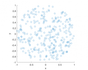
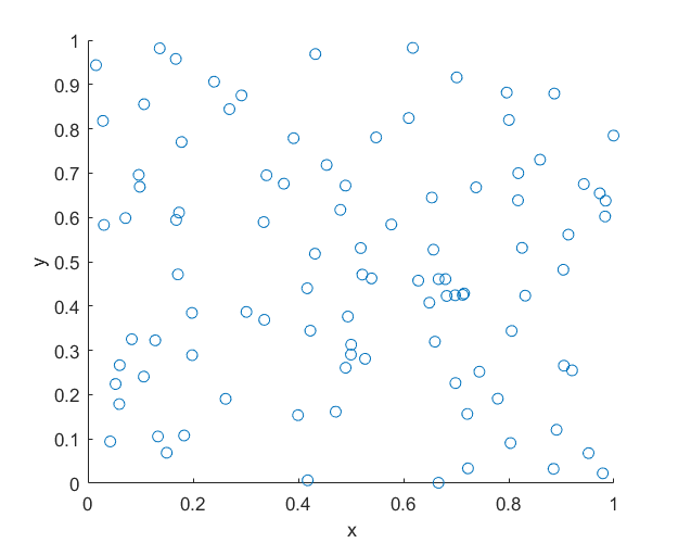
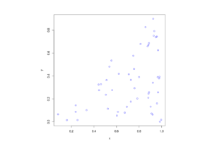
MATLAB
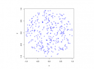
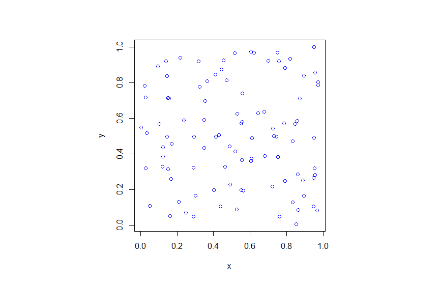
R
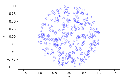
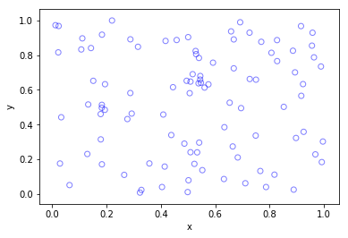
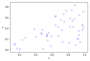
Python
Further reading
The topic of placing a single point uniformly on a general triangle is discussed in this StackExchange post. For the formulas, it cites the paper “Shape distributions” by Osada, Funkhouser, Chazelle and Dobkin”, where no proof is given.
I originally looked at placing single points in cells of a Dirichlet or Voronoi tesselation — terms vary. There is a lot of literature on this topic, particularly when the seeds of the cells form a Poisson point process. The references in the articles on Wikipedia and MathWorld are good starting points.
Correction
In a previous version of this blog, there was an error in the two Cartesian formula for randomly simulating a point in a triangle. This has been fixed, but the error never existed in the code.