

If you wanted to create a point process with repulsion, a reasonable first attempt would be to build off a Poisson point process by removing points according to some rule to ensure that no two points were within a certain distance of each other. Using this natural idea, Bertril Matérn proposed a family of repulsive point processes called Matérn hard-core point processes.
More specifically, Matérn proposed several points processes, including two types of hard-core point processes now called Type I and Type II. (Matérn proposed a third type, called Type III, but it’s considerably harder to simulate on a computer, as detailed in this article.) These types of hard-core point processes are completely different to the Matérn cluster point process.
As I discussed in a previous post, the Poisson point process may not be adequate for representing point phenomena whose points exhibit large degrees of repulsion or clustering. I already covered the Matérn and Thomas cluster point processes, which show distinct clustering in their configurations. In this post, I’ll cover Matérn hard-core point processes. The Type I point processes is the easier of the two, so I’ll start with that one.
Overview
Simulating Matérn hard-core point processes requires first simulating a homogeneous Poisson point process with an intensity \(\lambda>0\) on some simulation window, such as a rectangle, which is the simulation window I will use here. I have already written about simulating the homogeneous Poisson point processes on a rectangle and a disk, so those posts are good starting points.
Given the Poisson point process, the points then need to be thinned in such a manner to ensure that for each point, there is no other point within some fixed \(r>0\) of the point. This distance \(r>0\) is the radius of the hard core of each point.
I have already covered the point process operation of thinning. But it’s important to note here that in this construction a dependent thinning is being applied. (If I just applied an independent thinning, then the resulting point process will be another Poisson point process with no repulsion between points.)
Edge effects
The main trick behind sampling this point process is that it’s possible for points inside the simulation window to be thinned due to their closeness to points that are located outside the simulation window. In other words, points outside the simulation window can cause points inside the window to be thinned. (I discussed a very similar issue in the posts on the Matérn and Thomas cluster point processes.)
To remove these edge effects, the underlying Poisson point process must be simulated on an extended version of the simulation window. The points are then thinned according to a dependent thinning, which is covered in the next section. Then only the retained points inside the simulation window are kept and the remaining points are ignored. Consequently, the underling Poisson points are simulated on an extended window, but we only see the final points inside the simulation window.
To create the extended simulation window, we add a strip of width \(r\) all around the simulation window. Why? Well, the distance \(r\) is the maximum distance from the simulation window that another point (outside the simulation window) can exist, while still causing points inside the simulation window to be thinned. This means it is impossible for a hypothetical point beyond this distance (outside the extended window) to cause a point inside the simulation window to be thinned.
Dependent thinning rules
Type I
For each point inside the simulation window, check if there are any other points (including those in the extended window) within distance \(r\) of the point. If no, then keep the point. If yes, then remove the point and the points that are within distance \(r\) of the point. The remaining points inside the simulation window form a Matérn Type I point process.
This is a relatively simple thinning rule, which only requires calculating all the inter-point distances. But it is also a very strong thinning rule, meaning that it removes many points. Depending on the Poisson point process intensity \(\lambda\) and core radius \(r\), it is quite possible that all the points are removed, resulting in an empty configuration.
Now we examine the case when the thinning rule is not as strong.
Type II
To create Matérn Type II point process, we assign an independent uniform random variable to each point of the underlying Poisson point process defined on the extended window. In point process terminology, these random variables are called marks, resulting in a marked point process. In the the context of the Matérn Type II point process, these random random marks are usually called ages.
Then for each point in the simulation window, we consider all the points within distance \(r\) of the point. If this point is the youngest (or, equivalently, the oldest) point, then the point is kept. In other words, the point is only kept if its random mark is smaller (or larger) than the random marks of all the other points within distance \(r\) of the point. The remaining points inside the simulation window form a Matérn Type II point process.
Intensity expressions
Using point process and probability theory, one can derive mathematical expressions for the intensities (that is, the average density of points per unit area). These closed-form expressions can then be used to check that the correct number of points are being generated on average over many simulations.
Type I
The intensity of the Type I point process is given by
\[\mu_1=\lambda e^{-\lambda \pi r^2},\]
where \(\lambda \pi r^2\) is simply the area of the core.
Type II
The intensity of the Type II point process is given by
\[\mu_2=\frac{1}{\pi r^2}(1-e^{-\lambda \pi r^2}),\]
which can be written with the intensity of the the Type I point process as
\[\mu_2=\frac{1}{\pi r^2}(1-\frac{\mu_1}{\lambda}).\]
Code
I wrote the sampling code in MATLAB and Python, which are, as usual, very similar to each other. The code, which is is located here, simulates both Type I and II Matérn points processes. It also compares the empirical intensity to the the values given by the mathematical expressions in the previous section.
MATLAB
The MATLAB code is here.
Python
The Python code is here.
Results
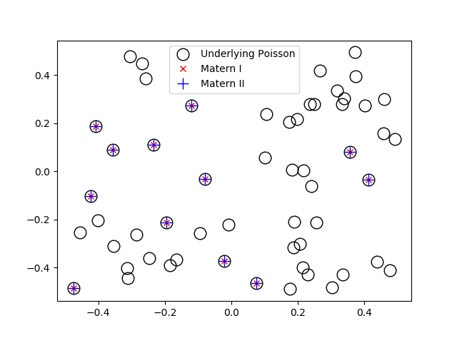
I have plotted single realizations of the Matern Type I and II point processes, as well as the underlying Poisson point process in the same window.
MATLAB
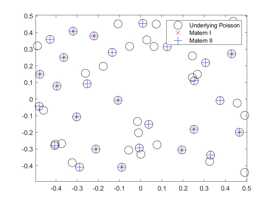
Python
Further reading
Matérn hard-core point processes are covered in standard books on the related fields of spatial statistics, point processes and stochastic geometry, such as the following: Spatial Point Patterns: Methodology and Applications with R by Baddeley, Rubak and Turner, on page 140; Statistical Analysis and Modelling of Spatial Point Patterns Statistics by Illian, Penttinen, Stoyan, amd Stoyan, Section 6.5.2, starting on page 388; and; Stochastic Geometry and its Applications by Chiu, Stoyan, Kendall and Mecke, Section 5.4, starting on page 176. The first two books are particularly good for beginners.
The aforementioned book Spatial Point Patterns: Methodology and Applications with R is written by spatial statistics experts Baddeley, Rubak and Turner. It covers the spatial statistics (and point process simulation) R-package spatstat., which has the functions rMaternI and rMaternII for simulating the two point processes respectively.