A Matérn cluster point process is a type of cluster point process, meaning that its randomly located points tend to form random clusters. (I skip the details here, but by using techniques from spatial statistics, it is possible to make the definition of clustering more precise.) This point process is an example of a family of cluster point processes known as Neyman-Scott point processes, which have been used in spatial statistics and telecommunications.
I should point out that the Matérn cluster point process should not be confused with the Matérn hard-core point process, which is a completely different type of point process. (For a research article, I have actually written code in MATLAB that simulates this type of point process.) Bertril Matérn proposed at least four types of point processes, and his name also refers to a specific type of covariance function used to define Gaussian processes.
Overview
Simulating a Matérn cluster point process requires first simulating a homogeneous Poisson point process with an intensity \(\lambda>0\) on some simulation window, such as a rectangle, which is the simulation window I will use here. Then for each point of this underlying point process, simulate a Poisson number of points with mean \(\mu>0\) uniformly on a disk with a constant radius \(r>0\). The underlying point process is sometimes called the parent (point) process, and its points are centres of the cluster disks.
The subsequent point process on all the disks is called daughter (point) process and it forms the clusters. I have already written about simulating the homogeneous Poisson point processes on a rectangle and a disk, so those posts are good starting points, and I will not focus too much on details for these steps.
Edge effects
The main challenge behind sampling this point process, which I originally forgot about in an earlier version of this post, is that it’s possible for daughter points to appear in the simulation window that come from parents points outside the simulation window. In other words, parents points outside the simulation window contribute to points inside the window.
To remove these edge effects, the point processes must be simulated on an extended version of the simulation window. Then only the daughter points within the simulation window are kept and the rest are removed. Consequently, the points are simulated on an extended window, but we only see the points inside the simulation window.
To create the extended simulation window, we can add a strip of width \(r\) all around the simulation window. Why? Well, the distance \(r\) is the maximum distance from the simulation window that a possibly contributing parent point (outside the simulation window) can exist, while still having daughter points inside the simulation window. This means it is impossible for a hypothetical parent point beyond this distance (outside the extended window) to generate a daughter point that can fall inside the simulation window.
Steps
Number of points
Simulate the underlying or parent Poisson point process on the rectangle with \(N_P\) parent points. Then for each parent point, simulate a Poisson number of offspring or daughter points, where each parent point now has \(D_i\) number of offspring points.
Then the total number of offspring points is simply \(N=D_1+\dots +D_{P}=\sum_{i=1}^{N_P}D_i \). The random variables \(P\) and \(D_i\) are Poisson random variables with respective means \(\lambda A\) and \(\mu\), where \(A\) is the area of the rectangular simulation window. To simulate these random variables in MATLAB, use the poissrnd function. To do this in R, use the standard function rpois. In Python, we can use either functions scipy.stats.poisson or numpy.random.poisson from the SciPy or NumPy libraries.
Locations of points
The points of the parent point process are randomly positioned by using Cartesian coordinates. For a homogeneous Poisson point process, the \(x\) and \(y\) coordinates of each point are independent uniform points, which is also the case for the binomial point process, covered in a previous post. The points of all the daughter point process are randomly positioned by using polar coordinates. For a homogeneous Poisson point process, the \(\theta\) and \(\rho\) coordinates of each point are independent variables, respectively with uniform and triangle distributions, which was covered in a previous post. Then we convert coordinates back to Cartesian form, which is easily done in MATLAB with the pol2cart function. In languages without such a function: \(x=\rho\cos(\theta)\) and \(y=\rho\sin(\theta)\).
Shifting all the points in each cluster disk
In practice (that is, in the code), all the daughter points are simulated in a disk with its centre at the origin. Then for each cluster disk, all the points have to be shifted to the origin is the center of the cluster, which completes the simulation step.
To use vectorization in the code, the coordinates of each cluster point are repeated by the number of daughters in the corresponding cluster by using the functions repelem in MATLAB, rep in R, and repeat in Python.
Code
I’ll now give some code in MATLAB, R and Python, which you can see are all very similar. It’s also located here.
MATLAB
The MATLAB code is located here.
R
The R code is located here.
Of course, as I have mentioned before, simulating a spatial point processes in R is even easier with the powerful spatial statistics library spatstat. The Matérn cluster point process is simulated by using the function rMatClust, but other cluster point processes, including Neyman-Scott types, are possible.
Python
The Pyhon code is located here.
Note: in previous posts I used the SciPy functions for random number generation, but now use the NumPy ones, but there is little difference, as SciPy builds off NumPy.
Julia
After writing this post, I later wrote the code in Julia. The code is here and my thoughts about Julia are here.
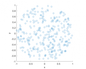
Results
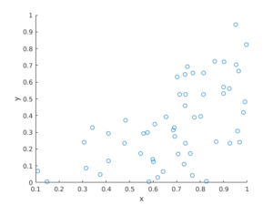
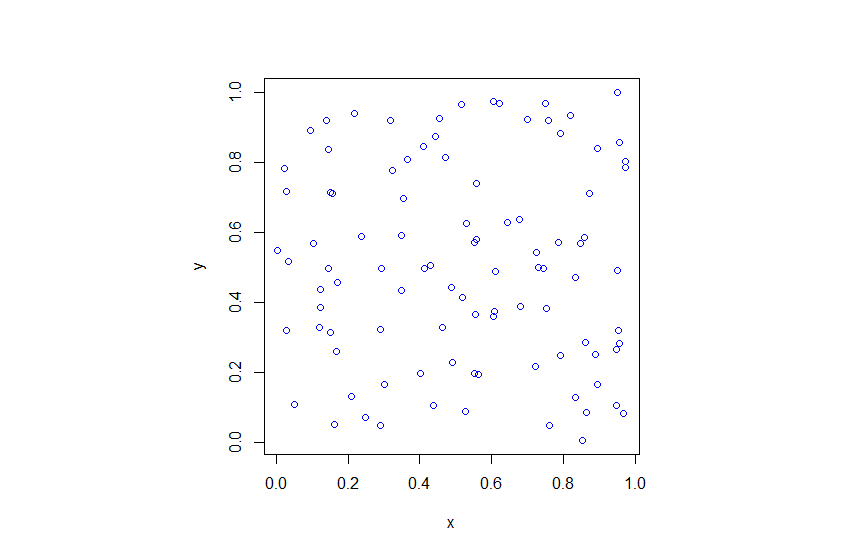
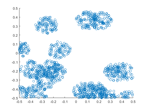
MATLAB
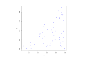
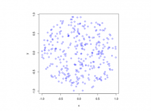
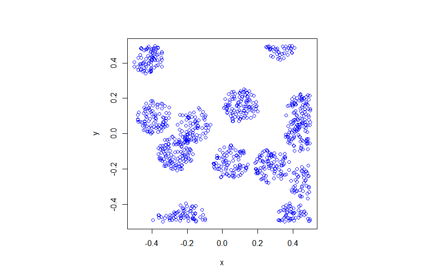
R
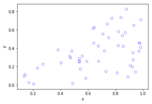
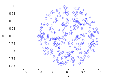
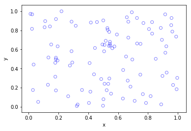
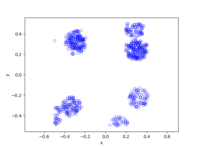
Python
Further reading
Matérn cluster point processes and more generally Neyman-Scott point processes are covered in standard books on the related fields of spatial statistics, point processes and stochastic geometry, such as the following: Spatial Point Patterns: Methodology and Applications with R by Baddeley, Rubak and Turner, on page 461; Statistical Analysis and Modelling of Spatial Point Patterns Statistics by Illian, Penttinen, Stoyan, amd Stoyan, Section 6.3.2, starting on page 370; Stochastic Geometry and its Applications by Chiu, Stoyan, Kendall and Mecke, on page 173; and; Statistical Inference and Simulation for Spatial Point Processes by Moller and Waagepetersen, in Section 5.3. I would probably recommend the first two books for beginners.
The Matérn point process has also appeared in models of wireless networks, which we covered in the book Stochastic Geometry Analysis of Cellular Networks by Błaszczyszyn, Haenggi, Keeler, and Mukherjee, Section 8.1.8.
I mentioned above the book Spatial Point Patterns: Methodology and Applications with R , which is written by spatial statistics experts Baddeley, Rubak and Turner. It covers the spatial statistics (and point process simulation) R-package spatstat.