Creating a reversible Markov chain using acceptance(-rejection)

The study of Markov chains is generally the study of their long term behaviour, which, under certain conditions, is captured by them having a unique stationary distribution. Stationarity is an important property. It is, in a sense, a local property of a Markov chain.

For a Markov chain, a more global property is something called reversibility. Markov chains with this property must possess a stationary distribution, which, we see below, is an immediate consequence of reversibility. Reversible Markov chains (or processes) with discrete time1Asmussen writes in his book Applied Probability and Queues:

In this book, we use the terminology that a Markov chain has discrete time and a Markov process has continuous time (the state space may be discrete or general). However, one should note that it is equally common to let “chain” refer to a discrete state space and “process” to a general one (time may be discrete or continuous).
are the cornerstone of Markov chain Monte Carlo (MCMC) methods.

In this post we look at how a reversible Markov chain is constructed from a non-reversible (but irreducible) Markov chain by introducing an acceptance-rejection step. This post complements another post I wrote on the Metropolis-Hastings algorithm.

Reversibility

A Markov process on state space \(\mathbb{X}\) with kernel \(K\) is (time) reversible with respect to the distribution \(\mu\) if the following holds

$$ \mu(x)K(x,y) = \mu (y) K(y,x)\quad x,y\in\mathbb{X}\,.$$

This reversibility condition is also called the detailed balance equation. If this condition is met, then the Markov process will have a stationary distribution \(\mu\). By summing over \(x\), we can verify this because we obtain

$$ \sum_{x\in\mathbb{X}}\mu(x)K(x,y) =\mu(y)\sum_{x\in\mathbb{X}} K(y,x)=\mu(y)\,.$$

This is just the balance equation, often written as \(\mu=K\mu\), which says that the transition kernel \(K\) has a stationary distribution \(\mu \).

First Markov chain

We consider a Markov chain with kernel \(J\) defined on a finite state space \(\mathbb{X}\). If the Markov chain is at state \(x\in \mathbb{X}\), it visits another state \(y\in \mathbb{X}\) with the probability \(J(x,y)\). This is a simple time-homogeneous finite Markov chain.

Irreducibility

For our Markov chain, we assume that every state \(x\) in \(\mathbb{X}\) where \(\pi(x)>0\) is reachable with positive probability in a single step. This implies the easy-to-achieve condition \(J(x,y)>0\) where \(\pi(x)>0\) for all points \(x,y \in \mathbb{X}\). This requirement is a stronger form of irreducibility.

Creating a new Markov chain with acceptance

We create a new Markov chain by introducing an acceptance step. For the Markov chain with kernel \(J\), we assume that each time step, after choosing the jump direction but before jumping, a biased coin is flipped . The success probability \(\alpha(x,y)\) depends on the current position \(x\in \mathbb{X}\) and the (potential) next position \(y\in \mathbb{X}\).

Transition kernel

For our new Markov chain, we can quickly reason the transition kernel \(M\). We first look at the off-diagonal elements of the kernel (matrix) \(M\). To go from state \(x\) and to another state \(y\neq x\), the probability is simply

$$ M(x,y) = \alpha(x,y) J(x,y), \quad x\neq y\,.$$

The transition matrix \(M\) needs to be stochastic, so the rows sum to one, so \(\sum_{y\in\mathbb{X}}M(x,y)=1\). That gives us the diagonal elements of \(M\), although their exact form is not needed to show reversibility.

\(\alpha(x,y)\) needs a symmetric function \(s(x,y)\)

For reversibility, we just need to swap rows and columns. Clearly we only need to look at the off-diagonal entries, which implies the requirement

$$ \pi(x)M(x,y) = \pi (y) M(y,x)\quad x\neq y\,.$$

Both sides are symmetric in \(x\) and \(y\), meaning they are equal to some non-negative symmetric \(s(x,y)=s(y,x)\). Looking at the right-hand side, we get

$$\begin{aligned}\pi(y) M(y,x)&=\pi(y)J(y,x) \alpha(y,x)\\ &= s(y,x)\,.\end{aligned}$$

This implies that the function \(\alpha\) is a non-negative function such that \(\alpha\leq 1\), to ensure it’s a probability, with the form

$$ \alpha(x,y)=\frac{s(x,y)}{\pi(x)J(x,y)}\,.$$

The only task remaining now is to choose a reasonable symmetric function \(s\) such that \(\alpha\leq 1\), ensuring \(\alpha\) is a probability. Of course, our choice for the symmetric function \(s\) should also be a function of the stationary distribution \(\pi\) and the underlying kernel \(J\).

Examples

I’ll give two principal examples of the symmetric function \(s(x,y)\). Working in reverse chronological order, I’ll give the simpler of the two examples first.

Barker

A somewhat natural example is

$$s(x,y) = \frac{\pi(x)J(x,y)\pi(y)J(y,x)}{\pi(x)J(x,y)+\pi(y)J(y,x)}\,.$$

This is clearly a symmetric function, which only has the terms \(\pi\) and \(J\). The acceptance probability becomes

$$\alpha(x,y) = \frac{\pi(y)J(y,x)}{\pi(x)J(x,y)+\pi(y)J(y,x)}\,.$$

A.A. Barker proposed this function in a 1965 paper as part of his PhD work in mathematical physics at the University of Adelaide. Barker had been inspired by a previous 1953 paper, which brings us to the next example.

Metropolis(-Rosenbluth-Rosenbluth-Teller-Teller)-Hastings

The now most important example is

$$s(x,y) = \min[\pi(x)J(x,y),\pi(y)J(y,x)]\,.$$

We can see that this is a symmetric function. The acceptance probability becomes

$$\alpha(x,y) = \min[1,\frac{\pi(y)J(y,x)}{\pi(x)J(x,y)}]\,.$$

This example is very famous in the world of Markov chain Monte Carlo methods. It is the main part of the so-called Metropolis-Hastings algorithm, which comes from a 1953 paper by Nicholas Metropolis, Arianna W. Rosenbluth, Marshall Rosenbluth, Augusta H. Teller, and Edward Teller (two husband-wife pairs), who looked at a special case, and a 1970 paper by W.K. Hastings, who generalized the method.

Further reading

Articles

Historical

The two important historical papers that gave the two examples for \(s(x,y)\) are:

  • 1965 – Barker – Monte Carlo calculations of the radial distribution functions for a proton-electron plasma;
  • 1953 – Metropolis, Rosenbluth, Rosenbluth, Teller, Teller – Equation of state calculations by fast computing machines.

This paper is also important:

  • 1970 – Hastings – Monte Carlo sampling methods using Markov chains and their applications.
Introductory

A good explanatory article about the Metropolis-Hastings algorithm is:

  • 1995 – Chib and Greenberg – Understanding the Metropolis-Hastings Algorithm.

I also recommend:

  • 2015 – Minh and Minh – Understanding the Hastings Algorithm;
  • 2016 – Robert – The Metropolis-Hastings algorithm;
  • 2017 – Gonçalves, Łatuszyński, Roberts – Barker’s algorithm for Bayesian inference with intractable likelihoods.
History

The history of this and related methods is described in the following article:

  • 2011 – Robert and Casella – A Short History of Markov Chain Monte Carlo: Subjective Recollections from Incomplete Data.

Incidentally, the first author, Christian P. Robert, writes on his blog about Markov chain Monte Carlo methods, such as the Metropolis-Hastings algorithm, as well as many other topics.

Books

Modern books on stochastic simulations and Monte Carlo methods will often detail this method. For example, see the Handbook of Monte Carlo Methods (Section 6.1) by Kroese, Taimre and Botev. The book Stochastic Simulation: Algorithms and Analysis by Asmussen and Glynn also covers the method in Chapter XIII, Section 3. (For my remark on reversibility, see Remark 3.2 in Asmussen and Glynn.) There is also the book Monte Carlo Strategies in Scientific Computing by Liu; see Chapter 5.

Websites

The web abounds with pages dedicated to explaining Markov chain Monte Carlo methods with the focus typically on the Metropolis-Hastings algorithm. I would try this following one because it gives a detailed explanation on how the Metropolis-Hastings algorithm works:

  • https://gregorygundersen.com/blog/2019/11/02/metropolis-hastings/

Poisson (stochastic) process

One of the most important stochastic processes is Poisson stochastic process, often called simply the Poisson process. In a previous post I gave the definition of a stochastic process (also called a random process) alongside some examples of this important random object, including counting processes.  The Poisson (stochastic) process is a counting process. This continuous-time  stochastic process is a highly studied and used object. It plays a key role in different probability fields, particularly those focused on stochastic processes such as stochastic calculus (with jumps) and the theories of Markov processes, queueingpoint processes (on the real line), and Levy processes.

The points in time when a Poisson stochastic process increases form a Poisson point process on the real line. In this setting the stochastic process and the point process can be considered two interpretations of the same random object.  The Poisson point process is often just called the Poisson process, but a Poisson point process can be defined on more generals spaces. In some literature, such as the theory of Lévy processes, a Poisson point process is called a Poisson random measure, differentiating the Poisson point process from the Poisson stochastic process. Due to the connection with the Poisson distribution, the two mathematical objects are named after Simeon Poisson, but he never studied these random objects.

The other important stochastic process is the Wiener process or Brownian (motion process), which I cover in another post. The Wiener process is arguably the most important stochastic process. I have written that post and the current one with the same structure and style, reflecting and emphasizing the similarities between these two fundamental stochastic process.

In this post I will give a definition of the homogenous Poisson process. I will also describe some of its key properties and importance. In future posts I will cover the history and generalizations of this stochastic process.

Definition

In the stochastic processes literature there are different definitions of the Poisson process. These depend on the settings such as the level of mathematical rigour. I give a mathematical definition which captures the main characteristics of this stochastic process.

Definition: Homogeneous Poisson (stochastic) process

An integer-valued stochastic process \(\{N_t:t\geq 0 \}\) defined on a probability space \((\Omega,\mathcal{A},\mathbb{P})\) is a homogeneous Poisson (stochastic) process if it has the following properties:

  1. The initial value of the stochastic process \(\{N_t:t\geq 0 \}\) is zero with probability one, meaning \(P(N_0=0)=1\).
  2. The increment \(N_t-N_s\) is independent of the past, that is, \(N_u\), where \(0\leq u\leq s\).
  3. The increment \(N_t-N_s\) is a Poisson variable with mean \(\lambda (t-s)\).

In some literature, the initial value of the stochastic process may not be given. Alternatively, it is simply stated as \(N_0=0\) instead of the more precise (probabilistic) statement given above.

Also, some definitions of this stochastic process include an extra property or two. For example, from the above definition, we can infer that increments of the homogeneous Poisson process are stationary due to the properties of the Poisson distribution. But a definition may include something like the following property, which explicitly states that this stochastic process is stationary.

  1. For \(0\leq u\leq s\), the increment \(N_t-N_s\) is equal in distribution to \(N_{t-s}\).

The definitions may also describe the continuity of the realizations of the stochastic process, known as sample paths, which we will cover in the next section.

It’s interesting to compare these defining properties with the corresponding ones of the standard Wiener stochastic process. Both stochastic processes build upon divisible probability distributions. Using this property, Lévy processes generalize these two stochastic processes.

Properties

The definition of the Poisson (stochastic) process means that it has stationary and independent increments. These are arguably the most important properties as they lead to the great tractability of this stochastic process. The increments are Poisson random variables, implying they can have only positive (integer) values.

The Poisson (stochastic) process exhibits closure properties, meaning you apply certain operations, you get another Poisson (stochastic) process. For example, if we sum two independent Poisson processes \(X= \{X_t:t\geq 0 \}\) and \(Y= \{Y_t:t\geq 0 \}\), then the resulting stochastic process \(Z=Z+Y = \{N_t:t\geq 0 \}\) is also a Poisson (stochastic) process. Such properties are useful for proving mathematical results.

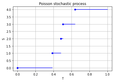
A single realization of a (homogeneous) Poisson stochastic process, where the blue marks show where the process jumps to the next value. In any finite time interval, there are a finite number of jumps.

Properties such as independence and stationarity of the increments are so-called distributional properties. But the sample paths of this stochastic process are also interesting. A sample path of a Poisson stochastic process is  almost surely non-decreasing, being constant except for jumps of size one. (The term almost surely comes from measure theory, but it means with probability one.) There are only finitely number of jumps in each finite time interval.

The homogeneous Poisson (stochastic) process has the Markov property, making it an example of a Markov process.  The homogenous Poisson process \(N=\{ N_t\}_{t\geq 0}\)s not a martingale. But interestingly, the stochastic process is \(\{ W_t – \lambda t\}_{t\geq 0}\) is a martingale. (Such relations have been used to study such stochastic processes with tools from martingale theory.)

Stochastic or point process?

The Poisson (stochastic) process is a discrete-valued stochastic process in continuous time. The relation these types of stochastic processes and point process is a subtle one. For example, David Cox and Valerie Isham write on page 3 of their monograph:

 The borderline between point processes and a  number of other kinds of stochastic process is not sharply defined. In particular, any stochastic process in continuous time in which the sample paths are step functions, and therefore any any process with a discrete state space, is associated with a point process, where a point is a time of transition or, more generally, a time of entry into a pre-assigned state or set of states. Whether it is useful to look at a particular process in this way depends on the purpose of the analysis.

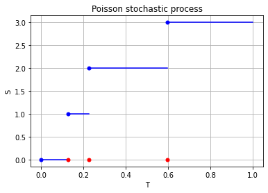
For the Poisson case, this association is presented in the diagram below. We can see the Poisson point process (in red) associated with the Poisson (stochastic) process (in blue) by simply looking at the time points where jumps occur.

A single realization of a (homogeneous) Poisson stochastic process (in blue). The jumps of the process form a (homogeneous) Poisson point process (in red) on the real line representing time.

Importance

Playing a prominent role in the theory of probability, the Poisson (stochastic) process is a highly important and studied stochastic process. It has connections to other stochastic processes and is central in queueing theory and random measures.

The Poisson process is a building block for more complex continuous-time Markov processes with discrete state spaces, which are used as mathematical models.  It is also essential in the study of jump processes and subordinators.

The Poisson (stochastic) process is a member of some important families of stochastic processes, including Markov processes, Lévy processes, and birth-death processes. This stochastic process also has many applications. For example, it plays a central role in quantitative finance. It is also used in the physical sciences as well as some branches of social sciences, as a mathematical model for various random phenomena.

Generalizations and modifications

For the Poisson (stochastic) process, the index set and state space are respectively the non-negative numbers and counting numbers, that is \(T=[0,\infty)\) and \(S=0, 1, \dots\), so it has a continuous index set but a discrete state space. Consequently, changing the state space, index set, or both offers an ways for generalizing and modifying the Poisson (stochastic) process.

Simulation

The defining properties of the Poisson stochastic process, namely independence and stationarity of increments, results in it being easy to simulate. The Poisson  stochastic process can be simulated provided random variables can be simulated or sampled according to a Poisson distributions, which I have covered in this and this post.

Simulating a Poisson stochastic process is similar to simulating a Poisson point process. (Basically, it is the same method in a one-dimensional setting.) But I will leave the details of sampling this stochastic process for another post.

Further reading

Here are some related links:

A very quick history of Wiener process and the Poisson (point and stochastic) process is covered in this talk by me.

In terms of books, the Poisson process has not received as much attention as the Wiener process, which is typically just called the Brownian (motion) process.  That said, any book covering queueing theory will cover the Poisson (stochastic) process.

More advanced readers can read about the Poisson (stochastic) process, the Wiener (or Brownian (motion)) process, and other Lévy processes:

On this topic, I recommend the introductory article:

  • 2004, Applebaum, Lévy Processes – From Probability to Finance and Quantum Groups.

This stochastic process is of course also covered in general books on stochastics process such as:


Wiener or Brownian (motion) process

One of the most important stochastic processes is the Wiener process or Brownian (motion) process. In a previous post I gave the definition of a stochastic process (also called a random process) with some examples of this important random object, including random walks. The Wiener process can be considered a continuous version of the simple random walk. This continuous-time stochastic process is a highly studied and used object. It plays a key role different probability fields, particularly those focused on stochastic processes such as stochastic calculus and the theories of Markov processes, martingales, Gaussian processes, and Levy processes.

The Wiener process is named after Norbert Wiener, but it is called the Brownian motion process or often just Brownian motion due to its historical connection as a model for Brownian movement in liquids, a physical phenomenon observed by Robert Brown. But the physical process is not true a Wiener process, which can be treated as an idealized model. I will use the terms Wiener process or Brownian (motion) process to differentiate the stochastic process from the physical phenomenon known as Brownian movement or Brownian process.

The Wiener process is arguably the most important stochastic process. The other important stochastic process is the Poisson (stochastic) process, which I cover in another post. I have written that and the current post with the same structure and style, reflecting and emphasizing the similarities between these two fundamental stochastic process.

In this post I will give a definition of the standard Wiener process. I will also describe some of its key properties and importance. In future posts I will cover the history and generalizations of this stochastic process.

Definition

In the stochastic processes literature there are different definitions of the Wiener process. These depend on the settings such as the level of mathematical rigour. I give a mathematical definition which captures the main characteristics of this stochastic process.

Definition: Standard Wiener or Brownian (motion) process

A real-valued stochastic process \(\{W_t:t\geq 0 \}\) defined on a probability space \((\Omega,\mathcal{A},\mathbb{P})\) is a standard Wiener (or Brownian motion) process if it has the following properties:

  1. The initial value of the stochastic process \(\{W_t:t\geq 0 \}\) is zero with probability one, meaning \(P(W_0=0)=1\).
  2. The increment \(W_t-W_s\) is independent of the past, that is, \(W_u\), where \(0\leq u\leq s\).
  3. The increment \(W_t-W_s\) is a normal variable with mean \(o\) and variance \(t-s\).

In some literature, the initial value of the stochastic process may not be given. Alternatively, it is simply stated as \(W_0=0\) instead of the more precise (probabilistic) statement given above.

Also, some definitions of this stochastic process include an extra property or two. For example, from the above definition, we can infer that increments of the standard Wiener process are stationary due to the properties of the normal distribution. But a definition may include something like the following property, which explicitly states that this stochastic process is stationary.

  1. For \(0\leq u\leq s\), the increment \(W_t-W_s\) is equal in distribution to \(W_{t-s}\).

The definitions may also describe the continuity of the realizations of the stochastic process, known as sample paths, which we will cover in the next section.

It’s interesting to compare these defining properties with the corresponding ones of the homogeneous Poisson stochastic process. Both stochastic processes build upon divisible probability distributions. Using this property, Lévy processes generalize these two stochastic processes.

Properties

The definition of the Wiener process means that it has stationary and independent increments. These are arguably the most important properties as they lead to the great tractability of this stochastic process. The increments are normal random variables, implying they can have both positive and negative (real) values.

The Wiener process exhibits closure properties, meaning you apply certain operations, you get another Wiener process. For example, if \(W= \{W_t:t\geq 0 \}\) is a Wiener process, then for a scaling constant \(c>0\), the resulting stochastic process \(\{W_{ct}/\sqrt{c}:t \geq 0 \}\)is also a Wiener process. Such properties are useful for proving mathematical results.

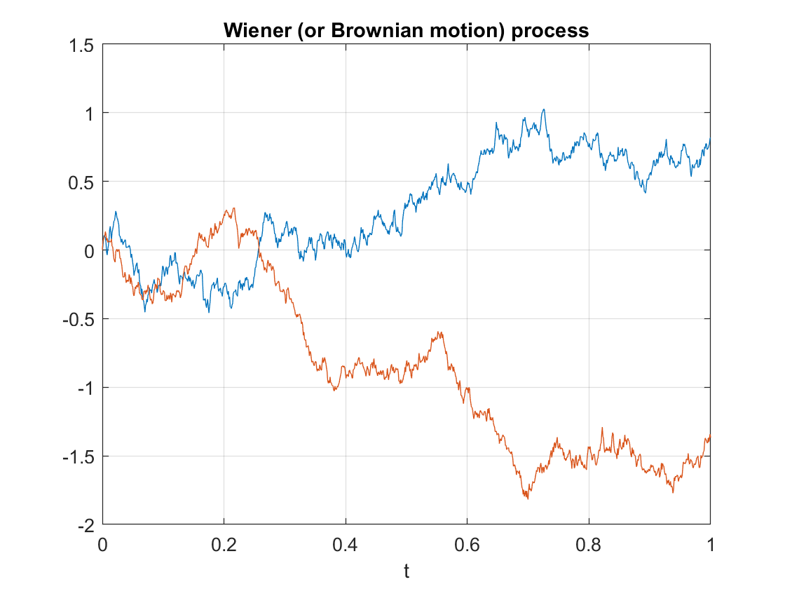
Two realizations of a Wiener (or Brownian motion) process. The sample paths are continuous (but non-differentiable) almost everywhere.

Properties such as independence and stationarity of the increments are so-called distributional properties. But the sample paths of this stochastic process are also interesting. A sample path of a Wiener process is continuous almost everywhere. (The term almost everywhere comes from measure theory, but it simply means that the only region where the property does not hold is mathematically negligible.) Despite the continuity of the sample paths, they are nowhere differentiable. (Historically, it was a challenge to find such a function, but a classic example is the Weierstrass function.)

The standard Wiener process has the Markov property, making it an example of a Markov process. The standard Wiener process \(W=\{ W_t\}_{t\geq 0}\) is a martingale. Interestingly, the stochastic process \(W=\{ W_t^2-t\}_{t\geq 0}\) is also a martingale. The Wiener process is a fundamental object in martingale theory.

There are many other properties of the Brownian motion process; see the Further reading section for, well, further reading.

Importance

Playing a main role in the theory of probability, the Wiener process is considered the most important and studied stochastic process. It has connections to other stochastic processes and is central in stochastic calculus and martingales. Its discovery led to the development to a family of Markov processes known as diffusion processes.

The Wiener process also arises as the mathematical limit of other stochastic processes such as random walks, which is the subject of Donsker’s theorem or invariance principle, also known as the functional central limit theorem.

The Wiener process is a member of some important families of stochastic processes, including Markov processes, Lévy processes, and Gaussian processes. This stochastic process also has many applications. For example, it plays a central role in quantitative finance. It is also used in the physical sciences as well as some branches of social sciences, as a mathematical model for various random phenomena.

Generalizations and modifications

For the Brownian motion process, the index set and state space are respectively the non-negative numbers and real numbers, that is \(T=[0,\infty)\) and \(S=[0,\infty)\), so it has both continuous index set and state space. Consequently, changing the state space, index set, or both offers an ways for generalizing or modifying the Wiener (stochastic) process.

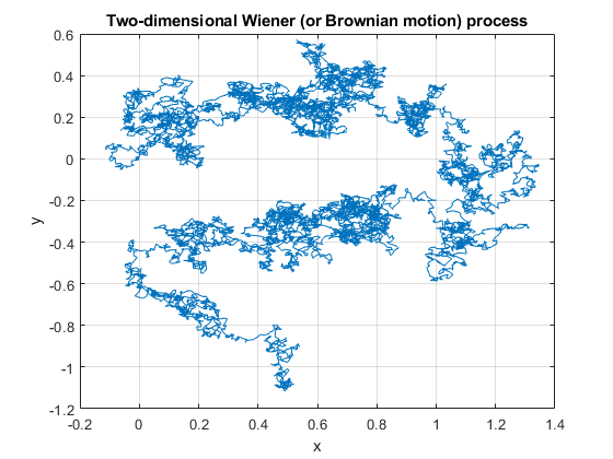
A single realization of a two-dimensional Wiener (or Brownian motion) process. Each vector component is an independent standard Wiener process.

Simulating

The defining properties of the Wiener process, namely independence and stationarity of increments, results in it being easy to simulate. The Wiener can be simulated provided random variables can be simulated or sampled according to a normal distribution. The main challenge is that the Wiener process is a continuous-time stochastic process, but computer simulations run in a discrete universe.

I will leave the details of sampling this stochastic process for another post.

Further reading

A very quick history of Wiener process and the Poisson (point) process is covered in this talk by me.

There are books almost entirely dedicated to the subject of the Wiener or Brownian (motion) process, including:

Of course the stochastic process is also covered in any book on stochastic calculus:

More advanced readers can read about the Wiener process, its descrete-valued cousin, the Poisson (stochastic) process, as well as other Lévy processes:

On this topic, I recommend the introductory article:

  • 2004, Applebaum, Lévy Processes – From Probability to Finance and Quantum Groups.

The Wiener process is of course also covered in general books on stochastic process such as:

Stochastic processes

I have written a few posts about point processes, which are mathematical objects that seek to represent points randomly scattered over some space. Arguably a much more popular random object is something called a stochastic process. This type of mathematical object, also frequently called a random process, is studied in mathematics. But the origins of stochastic processes stem from various phenomena in the real world.

Stochastic processes find applications representing some type of seemingly random change of a system (usually with respect to time). Examples include the growth of some population, the emission of radioactive particles, or the movements of financial markets. There are many types of stochastic processes with applications in various fields outside of mathematics, including the physical sciences, social sciences, finance, and engineering.

In this post I will cover the standard definition of a stochastic process. But first a quick reminder of some probability basics.

Probability basics

Random experiment

The mathematical field of probability arose from trying to understand games of chance. In these games, some random experiment is performed. A coin is flipped. A die is cast. A card is drawn. These random experiments give the initial intuition behind probability. Such experiments can be considered in more general or abstract terms.

A random experiment has the properties:

  1. Sample space: A sample space, denoted here by \(\Omega\), is the set of all (conceptually) possible outcomes of the random experiment;
  2. Outcomes: An outcome, denoted here by \(\omega\), is an element of the sample space \(\Omega\), meaning \(\omega \in \Omega\), and it is called a sample point or realization.
  3. Events: An event is a subset of the sample space \(\Omega\) for which probability is defined.
Examples
One die

Consider the rolling a traditional six-sided die with the sides numbered from \(1\) to \(6\). Its sample space is \(\Omega=\{1, 2, 3,4,5,6\}\). A possible event is an even number, corresponding to the outcomes \(\{2\}\), \(\{4\}\), and \(\{6\}\).

Two coins

Consider the flipping two identical coins, where each coin has a head appearing on one side and a tail on the other. We denote the head and tail respectively by \(H\) and \(T\). Then the sample space \(\Omega\) is all the possible outcomes, meaning \(\Omega=\{HH, TT, HT, TH\}\). A possible event is at least one head appearing, which corresponds to the outcomes \(\{HH\}\), \(\{HT\}\), and \(\{TH\}\).

Conversely, three heads \(\{HHH\}\), the number \(5\), or the queen of diamonds appearing are clearly not possible outcomes of flipping two coins, which means they are not elements of the sample space.

Modern probability approach

For a random experiment, we formalize what events are possible (or not) with a mathematical object called a \(\sigma\)-algebra. (It is also called \(\sigma\)-field.) This object is a mathematical set with certain properties with respect to set operations. It is a fundamental concept in measure theory, which is the standard approach for the theory of integrals. Measure theory serves as the foundation of modern probability theory.

In modern probability theory, if we want to define a random mathematical object, such as a random variable, we start with a random experiment in the context of a probability space or probability triple \((\Omega,\mathcal{A},\mathbb{P})\), where:

  1. \(\Omega\) is a sample space, which is the set of all (conceptually) possible outcomes;
  2. \(\mathcal{A}\) is a \(\sigma\)-algebra or \(\sigma\)-field, which is a family of events (subsets of \(\Omega\));
  3. \(\mathbb{P}\) is a probability measure, which assigns probability to each event in \(\mathcal{A}\).

To give some intuition behind this approach, David Williams says to imagine that Tyche, Goddess of Chance, chooses a point \(\omega\in\Omega\) at random according to the law \(\mathbb{P}\) such that an event \(A\in \mathcal{A}\) has a probability given by \(\mathbb{P}(A)\), where we understand probability with our own intuition. We can also choose \(\omega\in\Omega\) by using some physical experiment, as long as it is random.

With this formalism, mathematicians define random objects by using a certain measurable function or mapping that maps to a suitable space of mathematical objects. For example, a real-valued random variable is a measurable function from \(\Omega\) to the real line. To consider other random mathematical objects, we just need to define a measurable mapping from \(\Omega\) to a suitable mathematical space.

Definition

Stochastic process

Mathematically, a stochastic process is usually defined as a collection of random variables indexed by some set, often representing time. (Other interpretations exists such as a stochastic process being a random function.)

More formally, a stochastic process is defined as a collection of random variables defined on a common probability space \((\Omega,{\cal A}, \mathbb{P} )\), where \(\Omega\) is a sample space, \({\cal A}\) is a \(\sigma\)-algebra, and \(\mathbb{P}\) is a probability measure, and the random variables, indexed by some set \(T\), all take values in the same mathematical space \(S\), which must be measurable with respect to some \(\sigma\)-algebra \(\Sigma\).

Put another way, for a given probability space \(( \mathbb{P}, {\cal A}, \Omega)\) and a measurable space \((S, \Sigma)\), a stochastic process is a collection of \(S\)-valued random variables, which we can write as:

$$\{X(t):t\in T \}.$$

For each \(t\in T\), \(X(t)\) is a random variable. Historically, a point \(t\in T\) was interpreted as time, so \(X(t)\) is random variable representing a value observed at time \(t\).

Often the collection of random variables \(\{X(t):t\in T \}\) is denoted by simply a single letter such as \(X\).  There are different notations for stochastic processes. For example, a stochastic process can also be written as \(\{X(t,\omega):t\in T \}\), reflecting that is function of the two variables, \(t\in T\) and \(\omega\in \Omega\).

Index set

The set \(T\) is called the index set or parameter set of the stochastic process. Typically this set is some subset of the real line, such as the natural numbers or an interval. If the set is countable, such as the natural numbers, then it is a discrete-time stochastic process. Conversely, an interval for the index set gives a continuous-time stochastic process.

(If the index set is some two or higher dimensional Euclidean space or manifold, then typically the resulting stochastic or random process is called a random field.)

State space

The mathematical space \(S\) is called the state space of the stochastic process. The precise mathematical space can be any one of many different mathematical sets such as the integers, the real line, \(n\)-dimensional Euclidean space, the complex plane, or more abstract mathematical spaces. The different spaces reflects the different values that the stochastic process can take.

Sample function

A single outcome of a stochastic process is called a sample function, a sample path, or, a realization. It is formed by taking a single value of each random variable of the stochastic process. More precisely, if \(\{X(t,\omega):t\in T \}\) is a stochastic process, then for any point \(\omega\in\Omega\), the mapping
\[
X(\cdot,\omega): T \rightarrow S,
\]
is a sample function of the stochastic process \(\{X(t,\omega):t\in T \}\). Other names exist such as trajectory, and path function.

Examples

The range of stochastic processes is limitless, as stochastic processes can be used to construct new ones. Broadly speaking, stochastic processes can be classified by their index set and their state space. For example, we can consider a discrete-time and continuous-time stochastic processes.

There are some commonly used stochastic processes. I’ll give the details of a couple of very simple ones.

Bernoulli process

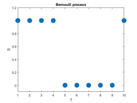
A very simple stochastic process is the Bernoulli process, which is a sequence of independent and identically distributed (iid) random variables. The value of each random variable can be one of two values, typically \(0\) and \(1\), but they could be also \(-1\) and \(+1\) or \(H\) and \(T\). To generate this stochastic process, each random variable takes one value,  say, \(1\) with probability \(p\) or the other value, say, \(0\) with probability \(1-p\).

We can can liken this stochastic process to flipping a coin, where the probability of a head is \(p\) and its value is \(1\), while the value of a tail is \(0\). In other words, a Bernoulli process is a sequence of iid Bernoulli random variables. The Bernoulli process has the counting numbers (that is, the positive integers) as its index set, meaning \(T=1,\dots\), while in this example the state space is simply \(S=\{0,1\}\).

A single realization of a Bernoulli process, one of the simplest stochastic processes. This discrete-time stochastic process only takes two values such as 0 and 1.

(We can easily generalize the Bernoulli process by having a sequence of iid variables with the same probability space.)

Random walks

A random walk is a type of stochastic process that is usually defined as sum of a sequence of iid random variables or random vectors in Euclidean space. Given random walks are formed from a sum, they are stochastic processes that evolve in discrete time. (But some also use the term to refer to stochastic processes that change in continuous time.)

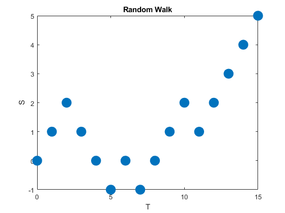
A classic example of this stochastic process is the simple random walk, which is based on a Bernoulli process, where each iid Bernoulli variable takes either the value positive one or negative one. More specifically, the simple random walk increases by one with probability, say, \(p\), or decreases by one with probability \(1-p\). The index set of this stochastic process is the natural numbers, while its state space is the integers.

A single realization of a simple (symmetric) random walk. This discrete-time stochastic process is a fundamental object in the history of probability theory.

Random walks can be defined in more general settings such as \(n\)- dimensional Euclidean space. There are other types of random walks, defined on different mathematical objects, such as lattices and groups, and in general they are highly studied and have many applications in different disciplines.

Markov processes

One important way for classifying stochastic processes is the stochastic dependence between random variables. For the Bernoulli process, there was no dependence between any random variable, giving a very simple stochastic process. But this is not a very interesting stochastic process.

A more interesting (and typically useful) stochastic process is one in which the random variables depend on each other in some way. For example, the next position of a random walk depends on the current position, which in turn depends on the previous position.

A large family of stochastic processes in which the next value depends on the current value are called Markov processes or Markov chains. (Both names are used. The term Markov chain is largely used when either the state space or index is discrete, but there does not seem to be an agreed upon convention. When I think Markov chain, I think discrete time.) The definition of a Markov process has a property that constrains the dependence between the random variables, as the next random variable only depends on the current random variable, and not all the previous random variables. This constraint on the dependence typically renders Markov processes more tractable than general stochastic processes.

It would be difficult to overstate the importance of Markov processes. Their study and application appear throughout probability, science, and technology.

Counting processes

A counting process is a stochastic process that takes the values of non-negative integers, meaning its state space is the counting numbers, and is non-decreasing. A simple example of a counting process is an asymmetric random walk, which increases by one with some probability \(p\) or remains the same value with probability \(1-p\). In other words, the accumulative sum of a Bernoulli process.  This is an example of a discrete-time counting process, but continuous-time ones also exist.

A counting process can be also interpreted as a counting as a random counting measure on the index set.

Two important stochastic processes

The most two important stochastic processes are the Poisson process and the Wiener process (often called Brownian motion process or just Brownian motion). They are important for both applications and theoretical reasons, playing fundamental roles in the theory of stochastic processes. In future posts I’ll cover both the Wiener process and the Poisson process.

Code

The code used to create the plots in this post is found here on my code repository. The code exists in both MATLAB and Python.

Further reading

There are many, many books covering the fundamentals of modern probability theory, including those (in roughly increasing order of difficulty) by Grimmett and Stirzaker, Karr, Rosenthal, Shiryaev, Durrett, and Billingsley. A very quick introduction is given in this web article.

The development of stochastic processes is one of the great achievements in modern mathematics. Researchers and practitioners have both studied them in great depth and found many applications for them. Consequently, there is no shortage of literature on stochastic processes. For example:

Finally, one of the main pioneers of stochastic processes was Joseph Doob. His seminal book was simply called Stochastic Processes.

Some remarks regarding “On the Laplace Transform of the Aggregate Discounted Claims with Markovian arrivals”

Google Scholar has requested me to make available a freely available copy of this published comment my former PhD supervisor and I wrote a few years ago:

  • Keeler and Taylor, Some remarks regarding “On the Laplace Transform of the Aggregate Discounted Claims with Markovian arrivals”

OK, Google Scholar, here’s the manuscript that we submitted, which is basically the same as the published version.

The comment and the original paper cover an insurance model (for aggregate claims) that uses a Markov arrival process. Such stochastic processes use matrix theory. But there was a small error in the original paper, where commutativity had been assumed, which is clearly not the case in general for matrices. Despite this error, the incorrect solution gave surprisingly accurate answers, so we investigated why that was.

Nothing groundbreaking here by us. We were just curious.