In previous posts I described how to simulate homogeneous Poisson point processes on a rectangle, disk and triangle. But here I will simulate an inhomogeneous or nonhomogeneous Poisson point process. (Both of these terms are used, where the latter is probably more popular, but I prefer the former.) For such a point process, the points are not uniformly located on the underlying mathematical space on which the Poisson process is defined. This means that certain regions will, on average, tend to have more (or less) points than other regions of the underlying space.
Basics
Any Poisson point process is defined with a non-negative measure called the intensity or mean measure. I make the standard assumption that the intensity measure \(\Lambda\) has a derivative \(\lambda(x,y)\). (I usually write a single \(x\) to denote a point on the plane, that is \(x\in \mathbb{R}^2\), but in this post I will write the \(x\) and \(y\) and coordinates separately.) The function \(\lambda(x,y)\) is often called the intensity function or just intensity, which I further assume is bounded, so \(\lambda(x,y)<\infty\) for all points in a simulation window \(W\). Finally, I assume that the simulation window \(W\) is a rectangle, but later I describe how to lift that assumption.
Number of points
To simulate a point process, the number of points and the point locations in the simulation window \(W\) are needed. For any Poisson point process, the number of points is a Poisson random variable with a parameter (that is, a mean) \(\Lambda(W)\), which under our previous assumptions is given by the integral
$$\Lambda(W)=\int_W \lambda(x,y)dxdy. $$
Assuming we can evaluate such an integral analytically or numerically, then the number of points is clearly not difficult to simulate.
Locations of points
The difficulty lies in randomly positioning the points. But a defining property of the Poisson point process is its independence, which allows us to treat each point completely independently. Positioning each point then comes down to suitably simulating two (or more) random variables for Poisson point processes in two (or higher) dimensions. Similarly, the standard methods used for simulating continuous random variables can be applied to simulating random point locations of a Poisson point process.
In theory, you can rescale the intensity function with the total measure of the simulation window, giving
$$f(x,y):=\frac{\lambda(x,y)}{\Lambda(W)}. $$
We can then interpret this rescaled intensity function \(f(x,y)\) as the joint probability density of two random variables \(X\) and \(Y\), because it integrates to one,
$$\int_W f(x,y)dxdy=1.$$
Clearly the method for simulating an inhomogeneous Poisson point process depends on the nature of the intensity function. For the inhomogeneous case, the random variables \(X\) and \(Y\) are, in general, not independent.
Transformation
To simulate an inhomogeneous Poisson point process, one method is to first simulate a homogeneous one, and then suitably transform the points according to deterministic function. For simple random variables, this transformation method is quick and easy to implement, if we can invert the probability distribution. For example, a uniform random variable \(U\) defined on the interval \((0,1)\) can be used to give an exponential random variable by applying the transformation \(h(u)= -(1/\lambda)\log(u)\), where \(\lambda>0\), meaning \(h(U)\) is an exponential random variable with parameter \(\lambda>0\) (or mean \(1/\lambda\)).
Similarly for Poisson point processes, the transformation approach is fairly straightforward in a one-dimensional setting, but generally doesn’t work easily in two (or higher) dimensions. The reason being that often we cannot simulate the random variables \(X\) and \(Y\) independently, which means, in practice, we need first to simulate one random variable, then the other.
It is a bit easier if we can re-write the rescaled intensity function or joint probability density \(f(x,y)\) as a product of single-variable functions \(f_X(x)\) and \(f_Y(y)\), meaning the random variables \(X\) and \(Y\) are independent. We can then simulate independently the random variables \(X\) and \(Y\), corresponding to the \(x\) and \(y\) coordinates of the points. But this would still require integrating and inverting the functions.
Markov chain Monte Carlo
A now standard way to simulate jointly distributed random variables is to use Markov chain Monte Carlo (MCMC), which we can also use to simulate the the \(X\) and \(Y\) random variables. Applying MCMC methods is simply applying random point process operations repeatedly to all the points. But this is a bit too tricky and involved. Instead I’ll use a general yet simpler method based on thinning.
Thinning
The thinning method is the arguably the simplest and most general way to simulate an inhomogeneous Poisson point process. If you’re unfamiliar with thinning, I recommend my previous post on thinning and the material I cite.
This simulation method is simply a type of acceptance-rejection method for simulating random variables. More specifically, it is the acceptance-rejection or rejection method, attributed to the great John von Neumann, for simulating a continuous random variable, say \(X\), with some known probability density \(f(x)\). The method accepts/retains or rejects/thins the outcome of each random variable/point depending on the outcome of a uniform random variable associated with each random variable/point.
The thinning or acceptance-rejection method is also appealing because it is an example of a perfect simulation method, which means the distribution of the simulated random variables or points will not be an approximation. This can be contrasted with typical MCMC methods, which, in theory, reach the desired distribution of the random variables in infinite time, which is clearly not possible in practice.
Simulating the homogeneous Poisson point process
First simulate a homogeneous Poisson point process with intensity value \(\lambda^*\), which is an upper bound of the intensity function \(\lambda(x,y)\). The simulation step is the easy part, but what value is \(\lambda^*\)?
I will use the maximum value that the intensity function \(\lambda(x,y)\) takes, which I denote by
$$ \lambda_{\max}:=\max_{(x,y)\in W}\lambda(x,y),$$
so I set \(\lambda^*=\lambda_{\max}\). Of course with \(\lambda^*\) being an upper bound, you can use any larger \(\lambda\)-value, so \(\lambda^*\geq \lambda_{\max}\), but that just means more points will need to be thinned.
Scientific programming languages have implemented algorithms that find or estimate minima of mathematical functions, meaning such an algorithm just needs to find the \((x,y)\) point that gives the minimum value of \(-\lambda(x,y)\), which corresponds to the maximum value of \(\lambda(x,y)\). What is very important is that the minimization procedure can handle constraints on the \(x\) and \(y\) values, which in our case of a rectangular simulation window \(W\) are sometimes called box constraints.
Thinning the Poisson point process
All we need to do now is to thin the homogeneous Poisson point process with the thinning probability function
$$1-p(x,y)=\frac{\lambda(x,y)}{\lambda^*}.$$
This will randomly remove the points so the remaining points will form a inhomogeneous Poisson point process with intensity function
$$ (1-p(x,y))\lambda^* =\lambda(x,y).$$
As a result, we can see that provided \(\lambda^*\geq \lambda_{\max}>0\), this procedure will give the right intensity function \(\lambda(x,y)\). I’ll skip the details on the point process still being Poisson after thinning, as I have already covered this in the thinning post.
Empirical check
You can run an empirical check by simulating the point process a large number (say \(10^3\) or \(10^4\)) of times, and collect statistics on the number of points. As the number of simulations increases, the average number of points should converge to the intensity measure \(\Lambda(W)\), which is given by (perhaps numerically) evaluating the integral
$$\Lambda(W)=\int_W \lambda(x,y)dxdy.$$
This is a test for the intensity measure, a type of first moment, which will work for the intensity measure of any point process. But for Poisson point processes, the variance of the number of points will also converge to intensity measure \(\Lambda(W)\), giving a second empirical test based on second moments.
An even more thorough test would be estimating an empirical distribution (that is, performing and normalizing a histogram) on the number of points. These checks will validate the number of points, but not the positioning of the points. In my next post I’ll cover how to perform these tests.
Results
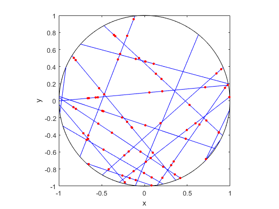
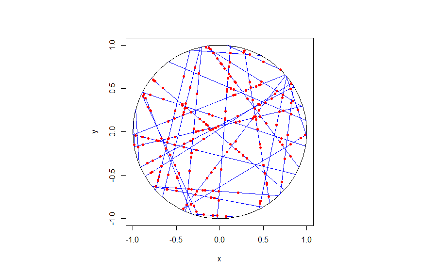
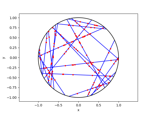
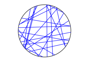
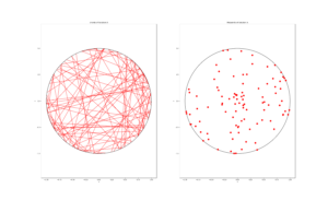
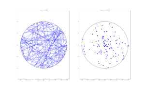
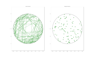
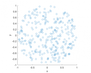
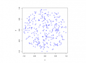
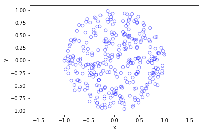
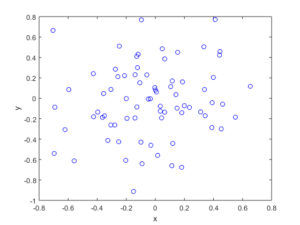
The homogeneous Poisson point process with intensity function \(\lambda(x)=100\exp(-(x^2+y^2)/s^2)\), where \(s=0.5\). The results look similar to those in the thinning post, where the thinned points (that is, red circles) are generated from the same Poisson point process as the one that I have presented here.
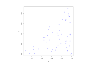
MATLAB
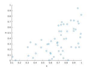
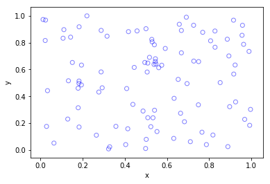
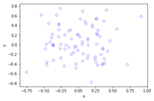
Python
Method extensions
We can extend the thinning method for simulating inhomogeneous Poisson point processes a couple different ways.
Using an inhomogeneous Poisson point process
The thinning method does not need to be applied to a homogeneous Poisson point process with intensity \(\lambda^*\). In theory, we could have simulated a suitably inhomogeneous Poisson point process with intensity function \(\lambda^*(x,y)\), which has the condition
$$ \lambda^*(x,y)\geq \lambda(x,y), \quad \forall (x,y)\in W .$$
Then this Poisson point process is thinned. But then we would still need to simulate the underlying Poisson point process, which often would be as difficult to simulate.
Partitioning the simulation window
Perhaps the intensity of the Poisson point process only takes two values, \(\lambda_1\) and \(\lambda_2\), and the simulation window \(W\) can be nicely divided or partitioned into two disjoints sets \(B_1\) and \(B_2\) (that is, \(B_1\cap B_2=\emptyset\) and \(B_1\cup B_2=W\)), corresponding to the subregions of the two different intensity values. The Poisson independence property allows us to simulate two independent Poisson point processes on the two subregions.
This approach only works for a piecewise constant intensity function. But if if the intensity function \(\lambda(x)\) varies wildly, the simulation window can be partitioned into subregions \(B_1\dots,B_m\) for different ranges of the intensity function \(\lambda(x)\). This allows us to simulate independent homogeneous Poisson point processes with different densities \(\lambda^*_1\dots, \lambda^*_m\), where for each subregion \(B_i\) we set
$$ \lambda^*_i:=\max_{x\in B_i}\lambda(x,y).$$
The resulting Poisson point processes are then suitably thinned, resulting in a more efficient simulation method. (Although I imagine the gain would often be small.)
Non-rectangular simulation windows
If you want to simulate on non-rectangular regions, which is not a disk or triangle, then the easiest way is to simulate a Poisson point process on a rectangle \(R\) that completely covers the simulation window, so \(W \subset R\subset \mathbb{R}^2\), and then set the intensity function \(\lambda \) to zero for the region outside the simulation window \(W\), that is \(\lambda (x,y)=0\) when \((x,y)\in R\setminus W\).
Further reading
In Section 2.5.2 of Stochastic Geometry and its Applications by Chiu, Stoyan, Kendall and Mecke, there is an outline of the thinning method that I used. The same simulation section appears in the previous edition by Kendall and Mecke, though these books in general have little material on simulation methods.
More details on the thinning method and its connection to acceptance-rejection sampling are given in Section 2.3 of the applications-oriented book Poisson Point Processes by Streit. The acceptance-rejection method is covered in, for example, books on Monte Carlo methods, including Monte Carlo Strategies in Scientific Computing by Liu (in Section 2.2 )and Monte Carlo Methods in Financial Engineering by Glasserman (in Section 2.2.2). This method and others for simulating generals random variable are covered in stochastic simulation books such as Uniform Random Variate Generation by Devroye and Stochastic Simulation: Algorithms and Analysis by Asmussen and Glynn.
Kroese and Botev have a good introduction to stochastic simulation in the edited collection Stochastic Geometry, Spatial Statistics and Random Fields : Models and Algorithms by Schmidt, where the relevant chapter (number 12) is also freely available online. And of course there are lectures notes on the internet that cover simulation material.
Code
All code from my posts, as always, can be found on the my GitHub repository. The code for this post is located here. You can see that the code is very similar to that of the thinning code, which served as the foundation for this code. (Note how we now keep the points, so in the code the > has become < on the line where the uniform variables are generated).
I have implemented the code in MATLAB and Python with an intensity function \(\lambda(x,y)=100\exp(-(x^2+y^2)/s^2)\), where \(s>0\) is a scale parameter. Note that in the minimization step, the box constraints are expressed differently in MATLAB and Python: MATLAB first takes the minimum values then the maximum values, whereas Python first takes the \(x\)-values then the \(y\)-values.
The code presented here does not have the empirical check, which I described above, but it is implemented in the code located here. For the parameters used in the code, the total measure is \(\Lambda(W)\approx 77.8068\), meaning each simulation will generate on average almost seventy-eight points.
I have stopped writing code in R for a couple of reasons, but mostly because anything I could think of simulating in R can already be done in the spatial statistics library spatstat. I recommend the book Spatial Point Patterns, co-authored by the spatstat’s main contributor, Adrian Baddeley.
MATLAB
I have used the fmincon function to find the point that gives the minimum of \(-\lambda(x,y)\).
%Simulation window parameters
xMin=-1;xMax=1;
yMin=-1;yMax=1;
xDelta=xMax-xMin;yDelta=yMax-yMin; %rectangle dimensions
areaTotal=xDelta*yDelta; %area of rectangle

s=0.5; %scale parameter

%Point process parameters
fun_lambda=@(x,y)(100*exp(-((x).^2+(y).^2)/s^2));%intensity function

%%%START -- find maximum lambda -- START %%%
%For an intensity function lambda, given by function fun_lambda,
%finds the maximum of lambda in a rectangular region given by
%[xMin,xMax,yMin,yMax].
funNeg=@(x)(-fun_lambda(x(1),x(2))); %negative of lambda
%initial value(ie centre)
xy0=[(xMin+xMax)/2,(yMin+yMax)/2];%initial value(ie centre)
%Set up optimization step
options=optimoptions('fmincon','Display','off');
%Find largest lambda value
[~,lambdaNegMin]=fmincon(funNeg,xy0,[],[],[],[],...
[xMin,yMin],[xMax,yMax],'',options);
lambdaMax=-lambdaNegMin;
%%%END -- find maximum lambda -- END%%%

%define thinning probability function
fun_p=@(x,y)(fun_lambda(x,y)/lambdaMax);

%Simulate Poisson point process
numbPoints=poissrnd(areaTotal*lambdaMax);%Poisson number of points
xx=xDelta*(rand(numbPoints,1))+xMin;%x coordinates of Poisson points
yy=xDelta*(rand(numbPoints,1))+yMin;%y coordinates of Poisson points

%calculate spatially-dependent thinning probabilities
p=fun_p(xx,yy);

%Generate Bernoulli variables (ie coin flips) for thinning
booleRetained=rand(numbPoints,1)<p; %points to be thinned

%x/y locations of retained points
xxRetained=xx(booleRetained); yyRetained=yy(booleRetained);

%Plotting
plot(xxRetained,yyRetained,'bo'); %plot retained points
xlabel('x');ylabel('y');
The box constraints for the optimization step were expressed as:
[xMin,yMin],[xMax,yMax]
Python
I have used the minimize function in SciPy.
import numpy as np; #NumPy package for arrays, random number generation, etc
import matplotlib.pyplot as plt #For plotting
from scipy.optimize import minimize #For optimizing
from scipy import integrate

#Simulation window parameters
xMin=-1;xMax=1;
yMin=-1;yMax=1;
xDelta=xMax-xMin;yDelta=yMax-yMin; #rectangle dimensions
areaTotal=xDelta*yDelta;

s=0.5; #scale parameter

#Point process parameters
def fun_lambda(x,y):
return 100*np.exp(-(x**2+y**2)/s**2); #intensity function

###START -- find maximum lambda -- START ###
#For an intensity function lambda, given by function fun_lambda,
#finds the maximum of lambda in a rectangular region given by
#[xMin,xMax,yMin,yMax].
def fun_Neg(x):
return -fun_lambda(x[0],x[1]); #negative of lambda

xy0=[(xMin+xMax)/2,(yMin+yMax)/2];#initial value(ie centre)
#Find largest lambda value
resultsOpt=minimize(fun_Neg,xy0,bounds=((xMin, xMax), (yMin, yMax)));
lambdaNegMin=resultsOpt.fun; #retrieve minimum value found by minimize
lambdaMax=-lambdaNegMin;
###END -- find maximum lambda -- END ###

#define thinning probability function
def fun_p(x,y):
return fun_lambda(x,y)/lambdaMax;

#Simulate a Poisson point process
numbPoints = np.random.poisson(lambdaMax*areaTotal);#Poisson number of points
xx = np.random.uniform(0,xDelta,((numbPoints,1)))+xMin;#x coordinates of Poisson points
yy = np.random.uniform(0,yDelta,((numbPoints,1)))+yMin;#y coordinates of Poisson points

#calculate spatially-dependent thinning probabilities
p=fun_p(xx,yy);

#Generate Bernoulli variables (ie coin flips) for thinning
booleRetained=np.random.uniform(0,1,((numbPoints,1)))<p; #points to be thinned

#x/y locations of retained points
xxRetained=xx[booleRetained]; yyRetained=yy[booleRetained];

#Plotting
plt.scatter(xxRetained,yyRetained, edgecolor='b', facecolor='none', alpha=0.5 );
plt.xlabel("x"); plt.ylabel("y");
plt.show();
The box constraints were expressed as:
(xMin, xMax), (yMin, yMax)
Julia
After writing this post, I later wrote the code in Julia. The code is here and my thoughts about Julia are here.