

In this post I’ll describe how to simulate or sample a homogeneous Poisson point process on the surface of a sphere. I have already simulated this point process on a rectangle, triangle disk, and circle.
Of course, by sphere, I mean the everyday object that is the surface of a three-dimensional ball, where this two-dimensional object is often denoted by \(S^2\). Mathematically, this is a generalization from a Poisson point process on a circle, which is slightly simpler than randomly positioning points on a disk. I recommend reading those two posts first, as a lot of the material presented here builds off them.
I have not needed such a simulation in my own work, but I imagine there are many reasons why you would want to simulate a Poisson point process on a sphere. As some motivation, we can imagine these points on a sphere representing, say, meteorites or lightning hitting the Earth.
The generating the number of points is not difficult. The trick is positioning the points on the sphere in a uniform way. As is often the case, there are various ways to do this, and I recommend this post, which lists the main ones. I will use two methods that I consider the most natural and intuitive ones, namely using spherical coordinates and normal random variables, which is what I did in the post on the circle.
Incidentally, a simple modification allows you to scatter the points uniformly inside the sphere, but you would typically say ball in mathematics, giving a Poisson point process inside a ball; see below for details.
Steps
As always, simulating a Poisson point process requires two steps.
Number of points
The number of points of a Poisson point process on the surface of a sphere of radius \(r>0\) is a Poisson random variable with mean \(\lambda S_2\), where \(S_2=4\pi r^2\) is the surface area of the sphere. (In this post I give some details for simulating or sampling Poisson random variables or, more accurately, variates.)
Locations of points
For any homogeneous Poisson point process, we need to position the points uniformly on the underlying space, which is in this case is the sphere. I now outline two different methods for doing this.
Method 1: Spherical coordinates
The first method is based on spherical coordinates \((\rho, \theta,\phi)\), where the radial coordinate \(\rho\geq 0\), and the angular coordinates \(0 \leq \theta\leq 2\pi\) and \(0\leq \phi \leq \pi\). The change of coordinates gives \(x=\rho\sin(\theta)\cos(\phi)\), \(y=\rho\sin(\theta)\sin(\phi)\), and \(z=\rho\cos(\phi)\).
Now we use Proposition 1.1 in this paper by Pitman and Ross. For each point, we generate two uniform variables \(V\) and \(\Theta\) on the respective intervals \((-1,1)\) and \((0,2\pi)\). Then we place the point with the Cartesian coordinates
$$X = r \sqrt{1-V^2} \cos\Theta, $$
$$Y = r \sqrt{1-V^2}\sin\Theta, $$
$$ Z=r V. $$
This method places a uniform point on a sphere with a radius \(r\).
How does it work?
I’ll skip the precise details, but give some interpretation of this method. The random variable \(\Phi := \arccos V\) is the \(\phi\)-coordinate of the uniform point, which implies \(\sin \Phi=\sqrt{1-V^2}\), due to basic trigonometric identities. The area element in polar coordinates is \(dA = \rho^2 \sin\phi d\phi d\theta \), which is constant with respect to \(\theta\). After integrating with respect to \(\phi\), we see that the random variable \(V=\cos\Phi\) needs to be uniform (instead of \(\Phi\)) to ensure the point is uniformly located on the surface.
Method 2: Normal random variables
For each point, we generate three standard normal or Gaussian random variables, say, \(W_x\), \(W_y\), and \(W_z\), which are independent of each other. (The term standard here means the normal random variables have mean \(\mu =0\) and standard deviation \(\sigma=1\).) The three random variables are the Cartesian components of the random point. We rescale the components by the Euclidean norm, then multiply by the radius \(r\), giving
$$X=\frac{rW_x}{(W_x^2+W_y^2+W_z^2)^{1/2}},$$
$$Y=\frac{rW_y}{(W_x^2+W_y^2+W_z^2)^{1/2}},$$
$$Z=\frac{rW_z}{(W_x^2+W_y^2+W_z^2)^{1/2}}.$$
These are the Cartesian coordinates of a point uniformly scattered on a sphere with radius \(r\) and a centre at the origin.
How does it work?
The procedure is somewhat like the Box-Muller transform in reverse. In the post on the circle setting, I gave an outline of the proof, which I recommend reading. The joint density of the normal random variables is from a multivariate normal distribution with zero correlation. This joint density is constant on the sphere, implying that the angle of the point \((W_x, W_y, W_z)\) will be uniformly distributed.
The vector formed from the normal variables \((W_x, W_y,W_z)\) is a random variable with a chi distribution. We can see that the vector from the origin to the point \((X,Y,Z)\) has length one, because we rescaled it with the Euclidean norm.
Plotting
Depending on your plotting software, the points may more resemble points on an ellipsoid than a sphere due to the different scaling of the x, y and z axes. To fix this in MATLAB, run the command: axis square. In Python, it’s not straightforward to do this, as it seems to lack an automatic function, so I have skipped it.
Results
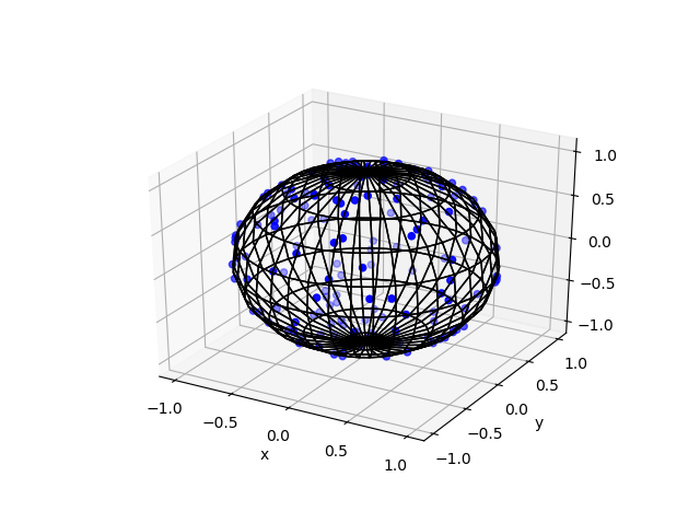
Here are some results produced by code written in MATLAB and Python. The blue points are the Poisson points on the sphere. I have used a surface plot (with clear faces) to illustrate the underling sphere in black.
MATLAB
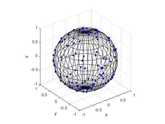
Python
Note: The aspect ratio in 3-D Python plots tends to squash the sphere slightly, but it is a sphere.
Code
The code for all my posts is located online here. For this post, the code in MATLAB and Python is here. In Python I used the library mpl_toolkits for doing 3-D plots.
Poisson point process inside the sphere
Perhaps you want to simulate a Poisson point process inside the ball. There are different ways we can do this, but I will describe just one way, which builds off Method 1 for positioning the points uniformly. (In a later post, I will modify Method 2, giving a way to uniformly position points inside the ball.)
For this simulation method, you need to make two simple modifications to the simulation procedure.
Number of points
The number of points of a Poisson point process inside a sphere of radius \(r>0\) is a Poisson random variable with mean \(\lambda V_3\), where \(V_3=4\pi r^3\) is the volume of the sphere.
Locations of points
We will modify Method 1 as outlined above. To sample the points uniformly in the sphere, you need to generate uniform variables on the unit interval \((0,1)\), take their cubic roots, and then, multiply them by the radius \(r\). (This is akin to the step of taking the square root in the disk setting.) The random variables for the angular coordinates are generated as before.
Further reading
I recommend this blog post, which discusses different methods for randomly placing points on spheres and inside spheres (or, rather, balls) in a uniform manner. (Embedded in two dimensions, a sphere is a circle and a ball is a disk.)
Our Method 2 for positioning points uniformly, which uses normal variables, comes from the paper:
- 1959, Muller, A note on a method for generating points uniformly on n-dimensional spheres.
This sampling method relies upon old observations that normal variables are connected to spheres and circles. I also found this post on a similar topic. Perhaps not surprisingly, the above paper is written by the same Muller behind the Box-Muller method for sampling normal random variables.
Update: The connection between the normal distribution and rotational symmetry has been the subject of some recent 3Blue1Brown videos on YouTube.
Here is some sample Python code for creating a 3-D scatter plot.
Hi. Why don’t you use the correct polar angle generator, which takes into account the fact that the elementary area on a sphere depends on the cosine of polar angle? If you do lots of points you will see that they are concentrated near poles, which is not a uniform poisson process. The correct algorithm should be something like theta=np.arccos(U*2-1), where U is a uniform between 0 and 1.
Thank you, Sergei. Good point. I was concentrating more on the second approach, so I missed that mistake. I’ve updated the method.
Thanks for posting this. Very useful to me in my current stage of research
If you want to make the python plot look more like the MATLAB plot you can use these settings to set the aspect ratio to 1×1:
## Plotting
fig = plt.figure(figsize=plt.figaspect(1)*2)
ax = plt.gca(projection=’3d’, proj_type = ‘ortho’)
Do you have any recommendations for implementing the K-function for points on a spherical surface?
Thank you, Ulysses, for your Python suggestion. I’ve updated that code.
As for (Ripley’s) K-function on spheres, well, whenever it’s spatial statistics, I look at Adrian Baddeley’s spatstat library in R, which is pretty well the best spatial statistics package around. For example:
https://rdrr.io/github/spatstat/spatstat.sphere/man/s2Kest.html
Note: “the theoretical value K(r) = 2 * pi * (1 – cos(r)) for a stationary Poisson process (where r is in radians).”
I imagine that the analytic result just falls out of the definition of the K function, which I believe is the second factorial moment measure with the test set, in this case, being a ball/disk on the sphere, meaning a spherical cap.
I hope that helps. Let me now if you need more help.
This is great. I got the K-function working on spherical surface data.
I do have one question that maybe you can help me with.
Are you aware of how to replicate the L-function on a sphere?
I know for a planar process L(r) = sqrt(K(r)/pi) -r
because that normalizes K(r) = pi*r^2 and sets the theoretical function to =0.
However, if K(r) = 2*pi*(1-cos(r)) on a sphere,
does that mean L(r) = acos(1-(K(r)/(2*pi)))-r?
I haven’t found a reference in the literature that explains how to calculate the L-function on a sphere. When I do this in r it looks somewhat plausible except it is missing the characteristic inhibition/regularization that is common in the beginning of planar L-functions.
Ripley’s K-function is a popular (and good) way to measure clustering/repulsion of points. You can then apply a transformation to the K-function, giving what some call the L-function. The transformation you gave, L(K(r),r) = sqrt(K(r)/pi) -r, is just one. (It’s a “centred” version.) I hadn’t actually seen that one before. I had only seen this one L(K) = sqrt(K/pi). Baddeley, Rubak, and Turner briefly discuss the different definitions of the L-function in Section 7.3.3 (page 207) of their book Spatial Point Patterns.
Also check out the book Statistical Inference and Simulation for Spatial Point Processes by Møller and Waagepetersen. In section 4.6, they give a general definition of a L-function as L(K(r),r)= [K(r)/w_d]^(1/d), where is d is the number of dimensions and w_d is the volume of a d-dimensional unit ball (see Section 3.1.3).
Remember on the sphere the variable r is the arc length (ie the distance over the sphere surface), not the radial distance. For a unit sphere, this means that values of r range from 0 to pi.
For your sphere problem, I am guessing you would set d=2, as the surface is two dimensions. But you would use the surface of a 3-dimensional unit ball. Recall the surface area of a sphere is 4\pi r^2, so the surface area of a unit sphere is sigma_3=4\pi. (This is just a normalization or scaling constant.)
Then for the (uncentred) definition of the L-function, I would guess L(r) = sqrt[K(r)/(4*pi)]=sqrt[(1 – cos(r))/2] for a homogeneous Poisson point process. Plugging in some numbers, we see that L(0)=0, L(pi/2)=1/2, and L(pi)=1.
But for your centred version, L(r) = sqrt[(1 – cos(r))/2]-r. But I would use L(r) = sqrt[(1 – cos(r))/2]-r/pi, so that you get nicer values for L(r).
Again, I stress I am guessing.
I hope that helps.
PS Here are two papers where they examine K-functions on the sphere:
https://onlinelibrary.wiley.com/doi/abs/10.1002/sta4.108
https://www.sciencedirect.com/science/article/abs/pii/S2211675314000487
The second one is easier to read (or more informal), but perhaps a touch too informal. For example, they do not use the term Poisson point process, but that is exactly the assumption they are making when they talk about something called complete spatial randomness (CSR), which is a term used less in spatial statistics and more in applied fields like ecology.
It seems the ability to study point patterns on spheres (using spatstat.sphere) is a relatively recent addition to spatstat, as noted in this update guide.
https://cran.r-project.org/web/packages/spatstat/vignettes/updates.pdf
Note how spatstat.sphere is still under development, which explains why there is no code (yet) for the L-function test on a sphere.
Your posts about poisson point process help a lot!!! Thank you!!!
Thanks 🙂
sir can you please help me out for plotting points on sphere using binomial point process
Well, a binomial point process is simpler than a Poisson point process. For the number of points, you don’t need to produce any random variables. You take the Poisson method (or code), and replace the Poisson random variable with the a fixed number of points, say, n.
For example, in my MATLAB code, you replace this line:
numbPoints=poissrnd(measureTotal*lambda);%Poisson number of points
with
numbPoints=10; %fixed number of points
In this example, the number of points is 10. The step is similar in the Python code — or whichever language. Here’s the link my code:
https://github.com/hpaulkeeler/posts/tree/master/PoissonSphere
Does that make sense?
Paul
Thanks for your great explanation! I have a question in mind, can we define a Poisson point process inside a cone also? I tried to do it but I face with some uncertainty. Like we can define a Cone in spherical coordinates as z = (1/tan(phi))*sqrt(x^2 + y^2) where phi must be constant (the angle cone makes with the z axis), sqrt(x^2 + y^2) = rho*sin(phi). I face problem when I want to limit points to be inside the cone space since the radius is changing w.r.t height. If you can introduce me a book or paper which has investigated this issue I would be thankful to you.
Thanks for your comment, Amin.
For your question, I think you first need to sample the z coordinate according Z=h*U^(1/3), where U is a uniform variable on (0,1) and h is the height. The volume is V=pi*r^2*h/3, where r is the radius of the circular base. The radius of the cross section at Z is linearly proportional to Z, so the volume is proportional to Z^3. Then based on the height Z, you sample the radius using a triangular distribution, so R=r*(Z/h)*sqrt(V), where V is another uniform variable on (0,1). Note that the gradient of the cone is just r/h. The angular coordinate Theta is simulated as before, uniformly on (0,2*pi). Then you convert R and Theta to Cartesian coordinates. This cone will be inverted with its tip at the origin.
I hope this helps.
For example, in MATLAB
%Simulation window parameters

h=2; %height of cone

r=1; %radius of base

xx0=0; yy0=0; zz0=0;%location of cone tip

volTotal=pi*r^2*h/3; %volume of cone
%Point process parameters
lambda=100; %intensity (ie mean density) of the Poisson process
%Simulate Poisson point process
numbPoints=poissrnd(volTotal*lambda);%Poisson number of points
zz=h*(rand(numbPoints,1)).^(1/3); %z coordinates
theta=2*pi*(rand(numbPoints,1)); %angular coordinates
rho=r*(zz/h).*sqrt(rand(numbPoints,1)); %radial coordinates
%Convert from polar to Cartesian coordinates
[xx,yy]=pol2cart(theta,rho); %x/y coordinates of Poisson points
%Shift tip of cone to (xx0,yy0,zz0)
xx=xx+xx0;
yy=yy+yy0;
zz=zz+zz0;
%Plotting
scatter3(xx,yy,zz);
xlabel('x');ylabel('y');
axis square;
If you search for how to sample a point uniformly inside a cone, you may find your answer on the web. Try googling uniformly located points, not necessarily a Poisson point process, which does have uniformly located points.
For example, this problem is discussed here with solution:
https://stackoverflow.com/questions/41749411/uniform-sampling-by-volume-within-a-cone