

In the previous post, I described how to simulate a Poisson line process, which in turn was done by using insight from an earlier post on the Bertrand paradox.
Now, given a Poisson line process, for each line, if we generate an independent one-dimensional Poisson point point process on each line, then we obtain an example of a Cox point process. Cox point processes are also known as doubly stochastic Poisson point processes. On the topic of names, Guttorp and Thorarinsdottir argue that it should be called the Quenouille point process, as Maurice Quenouille introduced an example of it before Sir David Cox, but I opt for the more common name.
Cox point proceesses
A Cox point process is a generalization of a Poisson point process. It is created by first considering a non-negative random measure, sometimes called a driving measure. Then a Poisson point process, which is independent of the random driving measure, is generated by using the random measure as its intensity or mean measure.
The driving measure of a Cox point process can be, for example, a non-negative random variable or field multiplied by a Lebesgue measure. In our case, the random measure is the underlying Poisson line process coupled with the Lebesgue measure on the line (that is, length).
Cox processes form a very large and general family of point processes, which exhibit clustering. In previous posts, I have covered two special cases of Cox point processes: the Matérn and Thomas cluster point processes. These are, more specifically, examples of a Neyman-Scott point process, which is a special case of a shot noise Cox point process. These two point processes are fairly easy to simulate, but that’s not the case for Cox point processes in general. Some are considerably easier than others.
Motivation
I will focus on simulating the Cox point process formed from a Poisson line process with homogeneous Poisson point processes. I do this for two reasons. First, it’s easy to simulate, given we can simulate a Poisson line process. Second, it has been used and studied recently in the mathematics and engineering literature for investigating wireless communication networks in cities, where the streets correspond to Poisson lines; for example, see these two preprints:
Incidentally, I don’t know what to call this particular Cox point process. A Cox line-point process? A Cox-Poisson line-point process? But it doesn’t matter for simulation purposes.
Method
We will simulate the Cox (-Poisson line-) point process on a disk. Why a disk? I suggest reading the previous posts on the Poisson line process and the Bertrand paradox for why the disk is a natural simulation window for line processes.
Provided we can simulate a Poisson line process, the simulation method is quite straightforward, as I have essentially already described it.
Line process
First simulate a Poisson line process on a disk. We recall that for each line of the line process, we need to generate two independent random variables \(\Theta\) and \(P\) describing the position of the line. The first random variable \(\Theta\) gives the line orientation, and it is a uniform random variable on the interval \((0,2\pi)\).
The second random variables \(P\) gives the distance from the origin to the disk edge, and it is a uniform random variable on the interval \((0,r)\), where \(r\) is the radius of the disk. The distance from the point \((\Theta, P)\) to the disk edge (that is, the circle) along the chord is:
$$Q=\sqrt{r^2-P^2}.$$
The endpoints of the chord (that is, the points on the disk edge) are then:
Point 1: \(X_1=P \cos \Theta+ Q\sin \Theta\), \(Y_1= P \sin \Theta- Q\cos \Theta\),
Point 2: \(X_2=P \cos \Theta- Q\sin \Theta\), \(Y_2= P \sin \Theta+Q \cos \Theta\).
The length of the line segment is \(2 Q\). We can say this random line is described by the point \((\Theta,P)\).
One-dimensional Poisson point process
For each line (segment) in the line process, simulate a one-dimensional Poisson point process on it. Although I have never discussed how to simulate a one-dimensional (homogeneous) Poisson point process, it’s essentially one dimension less than simulating a homogeneous Poisson point process on a rectangle.
More specifically, given a line segment \((\Theta,P)=(\theta,p)\), you simulate a homogeneous Poisson point process with intensity \(\mu\) on a line segment with length \(2 q\), where \(q=\sqrt{r^2-p^2}\). (I am now using lowercase letters to stress that the line is no longer random.) To simulate the homogeneous Poisson point process, you generate a Poisson random variable with parameter \(2 \mu q\).
Now you need to place the points uniformly on the line segment. To do this, consider a single point on a single line. For this point, generate a single uniform variable \(U\) on the interval \((-1,1)\). The tricky part is now getting the Cartesian coordinates right. But the above expressions for the endpoints suggest that the single random point has the Cartesian coordinates:
\(x=p \cos \theta+ U q\sin \theta\), \(y=p \sin \theta- U q\cos \theta\).
The two extreme cases of the uniform random variable \(U\) (that is, \(U=-1\) and \(U=1\)) correspond to the two endpoints of the line segment. We recall that \(Q\) is the distance from the midpoint of the line segment to the disk edge along the line segment, so it makes sense that we want to vary this distance uniformly in order to uniformly place a point on the line segment. This uniform placement step is done for all the points of the homogeneous Point process on that line segment.
You repeat this procedure for every line segment. And that’s it: a Cox point process built upon a Poisson line process.
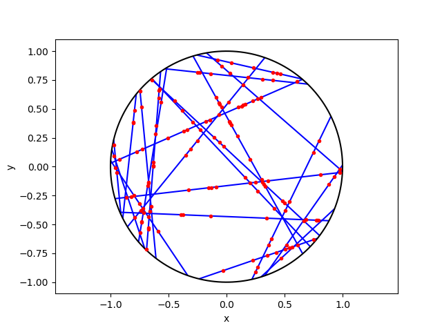
Results
MATLAB
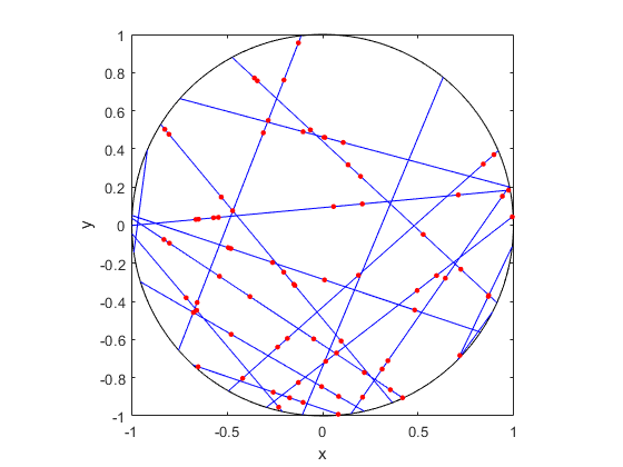
R
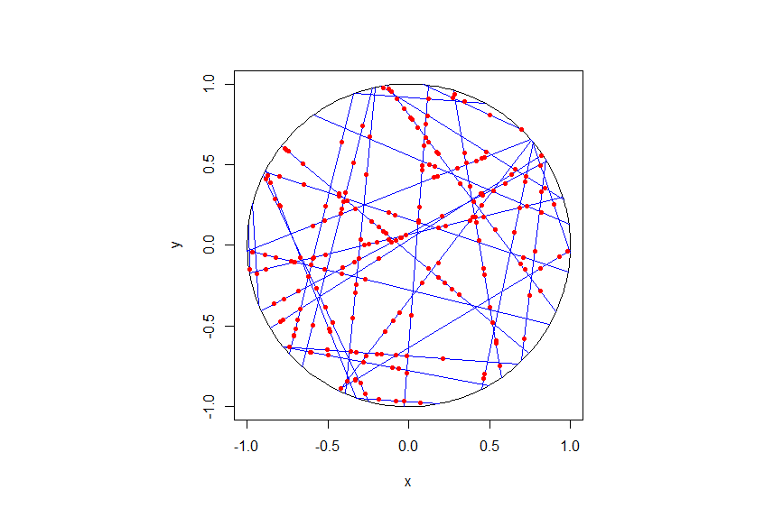
Python
Code
As always, the code from all my posts is online. For this post, I have written the code in MATLAB, R and Python.
Further reading
For the first step, the reading material is basically the same as that for the Poisson line process, which overlaps with that of the Bertrand paradox. For the one-dimensional Poisson point process, we can use the reading material on the homogeneous Poisson point process on a rectangle.
For general Cox point processes, I recommend starting with the following: Chapter 6 in the monograph Poisson Processes by Kingman; Chapter 5 in Statistical Inference and Simulation for Spatial Point Processes by Møller and Waagepetersen; and Section 5.2 in Stochastic Geometry and its Applications by Chiu, Stoyan, Kendall and Mecke. For a much more mathematical treatment, see Chapter 13 in Lectures on the Poisson Process by Last and Penrose, which is freely available online here.
For this particularly Cox point process, see the two aforementioned preprints, located here and here.