Simulating a Poisson point process on a disk

Sometimes one needs to simulate a Poisson point process on a disk. I know I often do. A disk or disc, depending on your spelling preference, is isotropic or rotationally-invariant, so a lot of my simulations of a Poisson point process happen in a circular simulation window when I am considering such a setting. For example, maybe you want to consider a single wireless receiver in a Poisson network of wireless transmitters, which only cares about the distance to a transmitter. Alternatively, maybe you want to randomly sprinkle a virtual cake. What to do? A Poisson point process on a disk is the answer.

In this post I will simulate a Poisson point process with intensity \(\lambda>0\) on a disk with radius \(r>0\).

Steps

The simulation steps are very similar to those in the previous post where I simulated a  homogeneous Poisson point process on a rectangle, and I suggest going back to that post if you are not familiar with the material. The main difference between simulation on a rectangle and a disk is the positioning of the points, but first we’ll look at the number of points.

Number of points

The number of points of a Poisson point process falling within a circle of radius \(r>0\) is a Poisson random variable with mean  \(\lambda A\), where \(A=\pi r^2\) is the area of the disk. As in the rectangular case, this is the most complicated part of the simulation procedure. But as long as your preferred programming language can produce (pseudo-)random numbers according to a Poisson distribution, you can simulate a homogeneous Poisson point process on a disk.

To do this in MATLAB,  use the poissrnd function with the argument \(\lambda A\). In R, it is done similarly with the standard  function rpois . In Python, we can use either the scipy.stats.poisson or numpy.random.poisson function from the SciPy or NumPy libraries.

Locations of points

We need to position all the points randomly and uniformly on a disk. In the case of the rectangle, we worked in Cartesian coordinates. It is then natural that we now work in polar coordinates.  I’ll denote the angular and radial coordinate respectively by \(\theta\) and \(\rho\). To generate the random angular (or \(\theta\)) values, we simply produce uniform random variables between zero and one, which is what all standard (pseudo-)random number generators do in programming languages. But we then multiply all these numbers by \(2\pi\), meaning that all the numbers now fall between \(0\) and \(2\pi\).

To generate the random radial (or \(\rho\)) values, a reasonable guess would be to do the same as before and generate uniform random variables between zero and one, and then multiply them by the disk radius \(r\). But that would be wrong.

Before multiplying uniform random variables by the radius, we must take the square root of all the random numbers. We then multiply them by the radius, generating random variables between \(0\) and \(r\). (We must take the square root because the area element of a sector or disk is proportional to the radius squared, and not the radius.) These random numbers do not have a uniform distribution, due to the square root, but in fact their distribution is an example of the triangular distribution, which is defined with three real-valued parameters \(a\), \(b\) and \(c\), and for our case, set \(a=0\) and \(b=c=r\).

In summary, if \(U\) and \(V\) are two independent uniform random variables on \((0,1)\), then random point located uniformly on a disk of radius \(r\) has the polar coordinates \((r\sqrt(U), 2\pi V)\).

From polar to Cartesian coordinates

That’s it. We have generated polar coordinates for points randomly and uniformly located in a disk. But to plot the points, often we have to convert coordinates back to Cartesian form. This is easily done in MATLAB with the pol2cart function. In languages without such a function, trigonometry comes to the rescue: \(x=\rho\cos(\theta)\) and \(y=\rho\sin(\theta)\).

Equal x and y axes

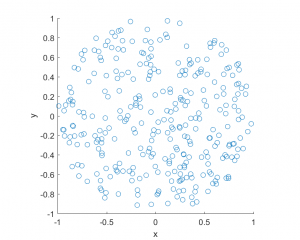
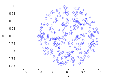
Sometimes the plotted points more resemble points on an ellipse than a disk due to the different scaling of the x and y axes. To fix this in MATLAB, run the command: axis square. In Python, set axis(‘equal’) in your plot; see this page for a demonstration.

Code

I’ll now give some code in MATLAB, R and Python, which, as you can see, are all very similar

MATLAB
%Simulation window parameters
r=1; %radius of disk
xx0=0; yy0=0; %centre of disk

areaTotal=pi*r^2; %area of disk
 
%Point process parameters
lambda=100; %intensity (ie mean density) of the Poisson process
 
%Simulate Poisson point process
numbPoints=poissrnd(areaTotal*lambda);%Poisson number of points
theta=2*pi*(rand(numbPoints,1)); %angular coordinates
rho=r*sqrt(rand(numbPoints,1)); %radial coordinates

%Convert from polar to Cartesian coordinates
[xx,yy]=pol2cart(theta,rho); %x/y coordinates of Poisson points

%Shift centre of disk to (xx0,yy0)
xx=xx+xx0;
yy=yy+yy0;
 
%Plotting
scatter(xx,yy);
xlabel('x');ylabel('y');
axis square;
R

Note: it is a bit tricky to write “<-” in the R code (as it automatically changes to the html equivalent in the HTML editor I am using), so I have usually used “=” instead of the usual “<-”.

#Simulation window parameters
r=1; #radius of disk
xx0=0; yy0=0; #centre of disk

areaTotal=pi*r^2; #area of disk

#Point process parameters
lambda=100; #intensity (ie mean density) of the Poisson process

#Simulate Poisson point process
numbPoints=rpois(1,areaTotal*lambda);#Poisson number of points
theta=2*pi*runif(numbPoints);#angular  of Poisson points
rho=r*sqrt(runif(numbPoints));#radial coordinates of Poisson points

#Convert from polar to Cartesian coordinates
xx=rho*cos(theta);
yy=rho*sin(theta);

#Shift centre of disk to (xx0,yy0)
xx=xx+xx0;
yy=yy+yy0;

#Plotting
par(pty="s")
plot(xx,yy,'p',xlab='x',ylab='y',col='blue');

Of course, with the amazing spatial statistics library spatstat, simulating a Poisson point process in R is even easier.

library("spatstat"); #load spatial statistics library
#create Poisson "point pattern" object
ppPoisson=rpoispp(lambda,win=disc(radius=r,centre=c(xx0,yy0))) 
plot(ppPoisson); #Plot point pattern object
#retrieve x/y values from point pattern object
xx=ppPoisson$x; 
yy=ppPoisson$y;

Actually, you can even do it all in two lines: one for loading the spatstat library and one for creating and plotting the point pattern object.

Python

Note: “lambda” is a reserved word in Python (and other languages), so I have used “lambda0” instead.

import numpy as np; #NumPy package for arrays, random number generation, etc
import matplotlib.pyplot as plt #for plotting

#Simulation window parameters
r=1;  #radius of disk
xx0=0; yy0=0; #centre of disk
areaTotal=np.pi*r**2; #area of disk

#Point process parameters
lambda0=100; #intensity (ie mean density) of the Poisson process

#Simulate Poisson point process
numbPoints = np.random.poisson(lambda0*areaTotal);#Poisson number of points
theta=2*np.pi*np.random.uniform(0,1,numbPoints); #angular coordinates 
rho=r*np.sqrt(np.random.uniform(0,1,numbPoints)); #radial coordinates 

#Convert from polar to Cartesian coordinates
xx = rho * np.cos(theta);
yy = rho * np.sin(theta);

#Shift centre of disk to (xx0,yy0) 
xx=xx+xx0; yy=yy+yy0;

#Plotting
plt.scatter(xx,yy, edgecolor='b', facecolor='none', alpha=0.5 );
plt.xlabel("x"); plt.ylabel("y");
plt.axis('equal');
Julia

After writing this post, I later wrote the code in Julia. The code is here and my thoughts about Julia are here.

Results

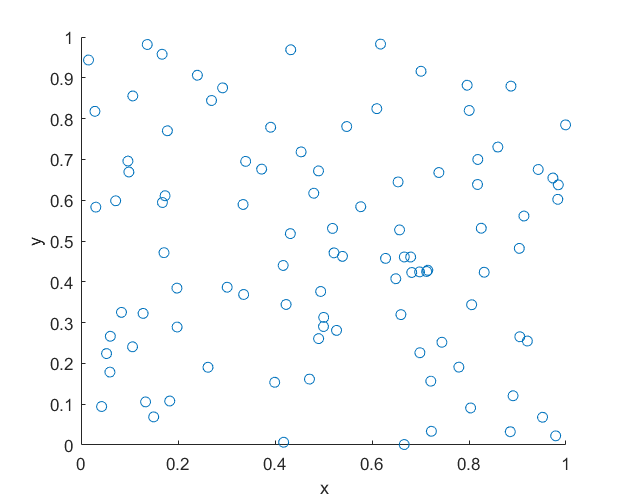
MATLAB
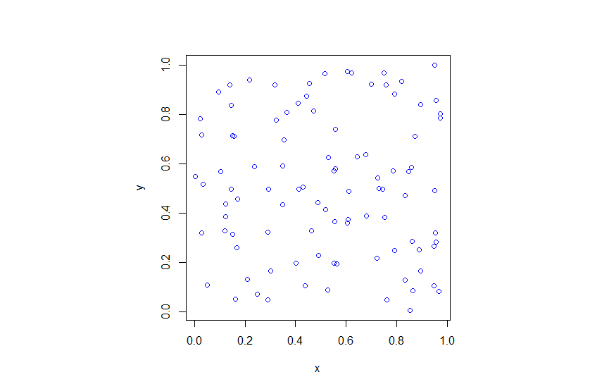
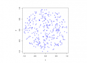
R 
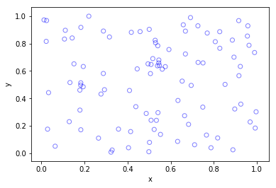
Python  
Further reading

The third edition of the classic book Stochastic Geometry and its Applications by Chiu, Stoyan, Kendall and Mecke details on page 54 how to uniformly place points on a disk, which they call the radial way. The same simulation section appears in the previous edition by Stoyan, Kendall and Mecke (Chiu didn’t appear as an author until the current edition), though these books in general have little material on simulation methods. There is the book Spatial Point Patterns: Methodology and Applications with R written by spatial statistics experts  Baddeley, Rubak and Turner, which covers the spatial statistics (and point process simulation) R-package spatstat.

Simulating a homogeneous Poisson point process on a rectangle

This is the first of a series of posts about simulating Poisson point processes. I’ll start with arguably the simplest Poisson point process on two-dimensional space, which is the homogeneous one defined on a rectangle. Let’s say that we we want to simulate a Poisson point process with intensity \(\lambda>0\) on a (bounded) rectangular region, for example, the rectangle \([0,w]\times[0,h]\) with dimensions \(w>0\) and \(h>0\) and area \(A=wh\). We assume for now that the bottom left corner of the rectangle is at the origin.

Steps

Number of points

The number of points in the rectangle  \([0,w]\times[0,h]\) is a Poisson random variable with mean \(\lambda A\). In other words, this random variable is distributed according to the Poisson distribution with parameter \(\lambda A\), and not just \(\lambda\), because the number of points depends on the size of the simulation region.

This is the most complicated part of the simulation procedure. As long as your preferred programming language can produce (pseudo-)random numbers according to a Poisson distribution, you can simulate a homogeneous Poisson point process. There’s a couple of different ways used to simulate Poisson random variables, but we will skip the details. In MATLAB, it is done by using the poissrnd function with the argument \(\lambda A\). In R, it is done similarly with the standard  function rpois . In Python, we can use either the scipy.stats.poisson or numpy.random.poisson function from the SciPy or NumPy libraries.

Location of points

The points now need to be positioned randomly, which is done by using Cartesian coordinates. For a homogeneous Poisson point process, the \(x\) and \(y\) coordinates of each point are independent uniform points, which is also the case for the binomial point process, covered in a previous post. For the rectangle \([0,w]\times[0,h]\), the \(x\) coordinates are uniformly sampled on the interval \([0,w]\), and similarly for the \(y\) coordinates. If the bottom left corner of rectangle is located at the point \((x_0,y_0)\), then we just have to shift the random \(x\) and \(y\) coordinates by respectively adding \(x_0\) and \(y_0\).

Every scientific programming language has a random uniform number generator because it is the default random number generator. In MATLAB, R and SciPy, it is respectively rand, runif and scipy.stats.uniform.

Code

Here is some code that I wrote for simulating a homogeneous Poisson point process on a rectangle. You will notice that in all the code samples the part that simulates the Poisson point process requires only three lines of code: one line for the number of points and two lines lines for the \(x\) and \(y\) coordinates  of the points.

MATLAB
%Simulation window parameters
xMin=0;xMax=1;
yMin=0;yMax=1;
xDelta=xMax-xMin;yDelta=yMax-yMin; %rectangle dimensions
areaTotal=xDelta*yDelta;

%Point process parameters
lambda=100; %intensity (ie mean density) of the Poisson process

%Simulate Poisson point process
numbPoints=poissrnd(areaTotal*lambda);%Poisson number of points
xx=xDelta*(rand(numbPoints,1))+xMin;%x coordinates of Poisson points
yy=yDelta*(rand(numbPoints,1))+yMin;%y coordinates of Poisson points

%Plotting
scatter(xx,yy);
xlabel('x');ylabel('y');
R

Note: it is a bit tricky to write “<-” in the R code (as it automatically changes to the html equivalent in the HTML editor I am using), so I have usually used “=” instead of the usual “<-”.

#Simulation window parameters
xMin=0;xMax=1;
yMin=0;yMax=1;
xDelta=xMax-xMin;yDelta=yMax-yMin; #rectangle dimensions
areaTotal=xDelta*yDelta;

#Point process parameters
lambda=100; #intensity (ie mean density) of the Poisson process

#Simulate Poisson point process
numbPoints=rpois(1,areaTotal*lambda);#Poisson number of points
xx=xDelta*runif(numbPoints)+xMin;#x coordinates of Poisson points
yy=yDelta*runif(numbPoints)+yMin;#y coordinates of Poisson points

#Plotting
plot(xx,yy,'p',xlab='x',ylab='y',col='blue');
Python

Note: “lambda” is a reserved word in Python (and other languages), so I have used “lambda0” instead.

import numpy as np
import scipy.stats
import matplotlib.pyplot as plt

#Simulation window parameters
xMin=0;xMax=1;
yMin=0;yMax=1;
xDelta=xMax-xMin;yDelta=yMax-yMin; #rectangle dimensions
areaTotal=xDelta*yDelta;

#Point process parameters
lambda0=100; #intensity (ie mean density) of the Poisson process

#Simulate Poisson point process
numbPoints = scipy.stats.poisson( lambda0*areaTotal ).rvs()#Poisson number of points
xx = xDelta*scipy.stats.uniform.rvs(0,1,((numbPoints,1)))+xMin#x coordinates of Poisson points
yy = yDelta*scipy.stats.uniform.rvs(0,1,((numbPoints,1)))+yMin#y coordinates of Poisson points
#Plotting
plt.scatter(xx,yy, edgecolor='b', facecolor='none', alpha=0.5 )
plt.xlabel("x"); plt.ylabel("y")
Julia

After writing this post, I later wrote the code in Julia. The code is here and my thoughts about Julia are here.

Results

MATLAB

PoissonMatlab

R

PoissonR

Python

PoissonPython

Higher dimensions

If you want to simulate a Poisson point process in a three-dimensional box (typically called a cuboid or rectangular prism), you just need two modifications.

For a box \([0,w]\times[0,h]\times[0,\ell]\), the number of points now a Poisson random variable with mean \(\lambda V\), where \(V= wh\ell\) is the volume of the box. (For higher dimensions, you need to use $n$-dimensional volume.)

To position the points in the box, you just need an additional uniform variable for the extra coordinate. In other words, the \(x\), \(y\) and \(z\) coordinates are uniformly and independently sampled on the respective intervals \([0,w]\), \([0,h]\), \([0,\ell]\). The more dimensions, the more uniform random variables.

And that’s it.

Further reading

For simulation of point processes, see, for example, the books Statistical Inference and Simulation for Spatial Point Processes by Møller and Waagepetersen, or Stochastic Geometry and its Applications by Chiu, Stoyan, Kendall and Mecke.

There are books written by spatial statistics experts such as Stochastic Simulation by Ripley and Spatial Point Patterns: Methodology and Applications with R by Baddeley, Rubak and Turner, where the second book covers the spatial statistics R-package spatstat. Kroese and Botev also have a good introduction in the edited collection Stochastic Geometry, Spatial Statistics and Random Fields : Models and Algorithms by Schmidt, where the relevant chapter (number 12) is also freely available online.

More general stochastic simulation books that cover relevant material include Uniform Random Variate Generation by Devroye and Stochastic Simulation: Algorithms and Analysis by Asmussen and Glynn.

Poisson point process

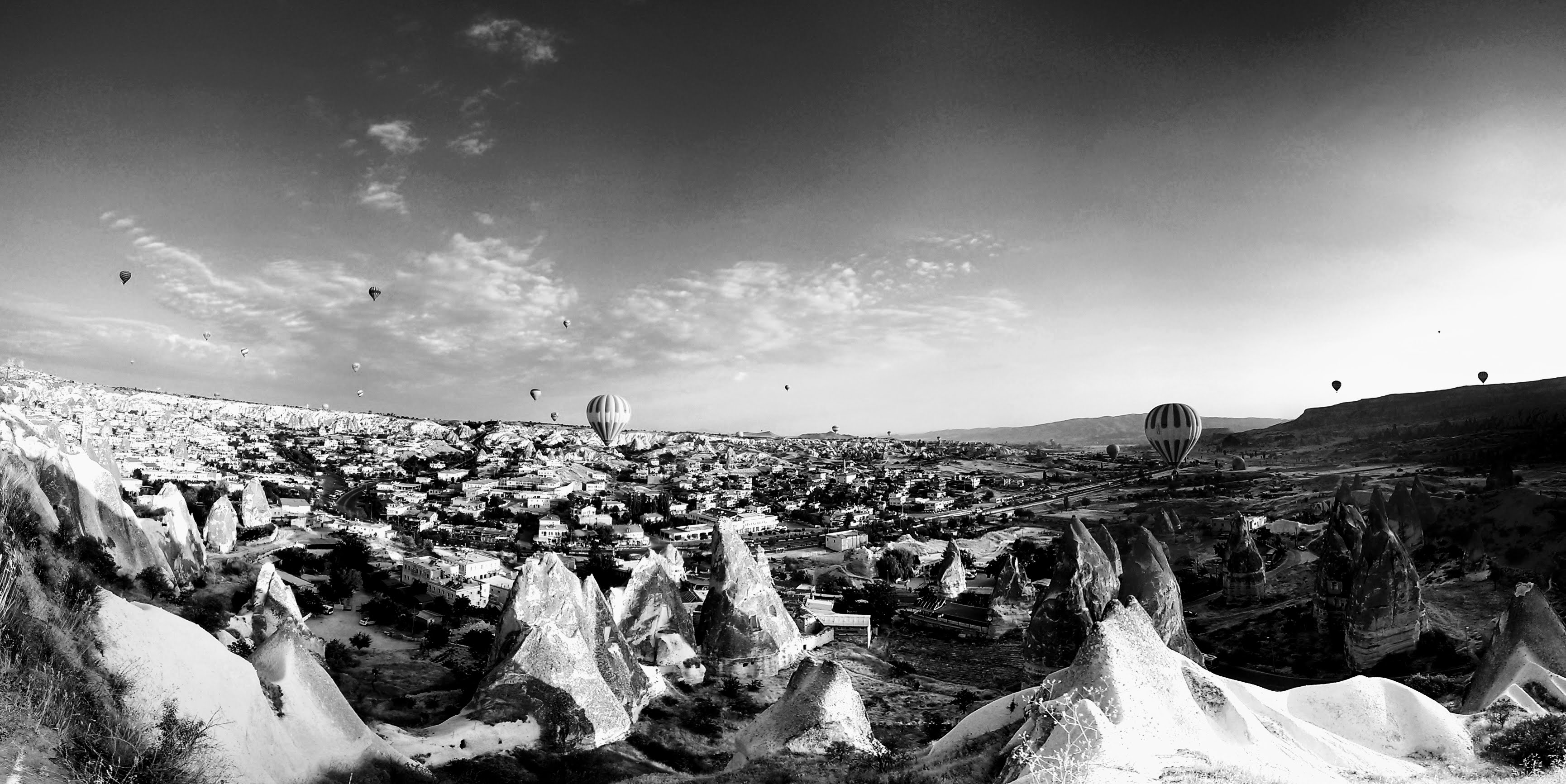
Balloons in scattered across a morning sky. Sand grains strewn on the ground. Seeds blown over a forest floor. Each of these phenomena can be represented mathematically as an object called a point process or random point field. Although it has a couple of mathematical interpretations, a point process is essentially just a collection of points randomly scattered on some mathematical space*, such as the real line, the Cartesian plane, a sphere, or more abstract spaces.

*The underlying mathematical space is sometimes called the carrier space or the state space, but the second term refers to something different from the state space used in the theory of stochastic processes.

The most important point process is the Poisson point process, which is one of the two most fundamental and studied mathematical objects in probability. (The other is the Wiener process or Brownian motion process, which is a type of random process or stochastic process, and it has been suggested by mathematicians such as John Kingman that the Poisson point process does not attract as much research attention as it should.) This point process can be defined on very general mathematical spaces, but usually the plane gives sufficient intuition. In this setting, each randomly located point can represent, for example, a star, a sand grain or a seed.

The most important defining property of the Poisson point process is that the numbers of points of the point process located in two (or more) non-overlapping (that is, disjoint) regions are two or more independent random variables. This property, sometimes called independent scattering or complete independence, explains the tremendous tractability of this point process, and it is used alongside the property that the random variables have Poisson distributions to define the Poisson point process.

To define a Poisson point process on some mathematical space, only a single mathematical object is needed. This object is applied to a region (or subset) of the underlying space on which the Poisson point process is defined, and returns a non-negative number. This object is a type of measure from measure theory, so it is called the mean measure or intensity measure. The mean measure can be interpreted as the mean or average number of points of a Poisson point process being located in a region of the underlying space.

Definition of a Poisson point process

A point process \(N\) defined on some underlying space \(S\) is a Poisson point process with intensity measure \(\Lambda\) if it has the two following properties:

1 The number of points in a bounded Borel set \(B \subset S\) is a Poisson random variable with mean \(\Lambda(B)\).

2 The number of points in \(n\) disjoint Borel sets forms \(n\) independent random variables.

A simple example of a mean measure of a Poisson point process is when the mean measure is given by the product of a non-negative constant and the area or volume of the region. The constant, often denoted by \(\lambda\), is known as the intensity or rate, which is often can be interpreted as the average density of points. In this setting, the average density does not vary over the underlying space, so the resulting point process is called a homogeneous Poisson point process or uniform Poisson point process, which is the simplest example of a Poisson point process.

If the intensity does change over the underlying space, meaning it is spatially dependent, then the terms inhomogeneous Poisson point process or nonhomogeneous Poisson point process are used. It is usually assumed that the intensity measure \(\Lambda\) has a derivative \(\lambda\), so it can be written as an integral:

$$\Lambda(B)=\int_B \lambda(x) dx, $$

where the set \(B\) is some subregion of the underlying state space \(S\). (As per standard probability assumptions, the set \(B\) has to be Borel measurable, but we do not focus on such details here.)

The Poisson point process is the cornerstone of fields where randomness meets geometry, such as spatial statistics, geometric probability and stochastic geometry. Researchers, scientists, and engineers have proposed using the Poisson point process to model various objects randomly positioned. In recent years, it has been used extensively to mathematically model the locations of transmitters and receivers in wireless communication networks such as cellular or mobile phone networks.

As a mathematical model, the Poisson point process should be used to represent objects or phenomena that have little or, ideally, zero interaction among the points. If that’s not the case, then the Poisson point process can also serve as a null-hypothesis model in statistics, whose rejection implies there is sufficiently strong interaction among the points. For example, the stars influence each other, undoubtedly, through gravity, and trees rely upon absorbing water in their vicinity through root systems, suggesting that non-Poisson models would be more suitable for representing these two examples. Other more sophisticated point processes that incorporate such point interaction have been developed. Many of these point processes build off the Poisson point process.

The Poisson point process is often called simply the Poisson process, where it can be confused with the related stochastic process of the same name. This Poisson process is a continuous-time discrete-valued stochastic process. The points in time where this stochastic process changes (or jumps) form the points of a Poisson point process on the real line. Depending on the literature, interpretation and preference, the Poisson point process is also called the Poisson random field and Poisson random measure.

The Poisson point process is a highly useful and used random object. But we now need to simulate it on a computer, which will be the subject of a future post.

Further reading

The Wikipedia article is a good starting point. The best book on the Poisson point process is the monograph Poisson Processes by Kingman. A recent and more theoretical book is Lecture Notes on the Poisson Process by Last and Penrose (the manuscript is freely available online here). More applied books include the classic Stochastic Geometry and its Applications by Chiu, Stoyan, Kendall and Mecke, and Statistical Inference and Simulation for Spatial Point Processes by Møller and Waagepetersen.

In recent years, there have been various books applying the Poisson point process to wireless networks, which include the two-volume Stochastic geometry and Wireless Networks by Baccelli and Błaszczyszyn, and Stochastic geometry for Wireless Networks by Haenggi. Much more recently, some colleagues and I contributed to this literature with Stochastic Geometry Analysis of Cellular Networks by Błaszczyszyn, Haenggi, Keeler, and Mukherjee.