

This is the first of a series of posts about simulating Poisson point processes. I’ll start with arguably the simplest Poisson point process on two-dimensional space, which is the homogeneous one defined on a rectangle. Let’s say that we we want to simulate a Poisson point process with intensity \(\lambda>0\) on a (bounded) rectangular region, for example, the rectangle \([0,w]\times[0,h]\) with dimensions \(w>0\) and \(h>0\) and area \(A=wh\). We assume for now that the bottom left corner of the rectangle is at the origin.
Steps
Number of points
The number of points in the rectangle \([0,w]\times[0,h]\) is a Poisson random variable with mean \(\lambda A\). In other words, this random variable is distributed according to the Poisson distribution with parameter \(\lambda A\), and not just \(\lambda\), because the number of points depends on the size of the simulation region.
This is the most complicated part of the simulation procedure. As long as your preferred programming language can produce (pseudo-)random numbers according to a Poisson distribution, you can simulate a homogeneous Poisson point process. There’s a couple of different ways used to simulate Poisson random variables, but we will skip the details. In MATLAB, it is done by using the poissrnd function with the argument \(\lambda A\). In R, it is done similarly with the standard function rpois . In Python, we can use either the scipy.stats.poisson or numpy.random.poisson function from the SciPy or NumPy libraries.
Location of points
The points now need to be positioned randomly, which is done by using Cartesian coordinates. For a homogeneous Poisson point process, the \(x\) and \(y\) coordinates of each point are independent uniform points, which is also the case for the binomial point process, covered in a previous post. For the rectangle \([0,w]\times[0,h]\), the \(x\) coordinates are uniformly sampled on the interval \([0,w]\), and similarly for the \(y\) coordinates. If the bottom left corner of rectangle is located at the point \((x_0,y_0)\), then we just have to shift the random \(x\) and \(y\) coordinates by respectively adding \(x_0\) and \(y_0\).
Every scientific programming language has a random uniform number generator because it is the default random number generator. In MATLAB, R and SciPy, it is respectively rand, runif and scipy.stats.uniform.
Code
Here is some code that I wrote for simulating a homogeneous Poisson point process on a rectangle. You will notice that in all the code samples the part that simulates the Poisson point process requires only three lines of code: one line for the number of points and two lines lines for the \(x\) and \(y\) coordinates of the points.
MATLAB
%Simulation window parameters
xMin=0;xMax=1;
yMin=0;yMax=1;
xDelta=xMax-xMin;yDelta=yMax-yMin; %rectangle dimensions
areaTotal=xDelta*yDelta;

%Point process parameters
lambda=100; %intensity (ie mean density) of the Poisson process

%Simulate Poisson point process
numbPoints=poissrnd(areaTotal*lambda);%Poisson number of points
xx=xDelta*(rand(numbPoints,1))+xMin;%x coordinates of Poisson points
yy=yDelta*(rand(numbPoints,1))+yMin;%y coordinates of Poisson points

%Plotting
scatter(xx,yy);
xlabel('x');ylabel('y');
R
Note: it is a bit tricky to write “<-” in the R code (as it automatically changes to the html equivalent in the HTML editor I am using), so I have usually used “=” instead of the usual “<-”.
#Simulation window parameters
xMin=0;xMax=1;
yMin=0;yMax=1;
xDelta=xMax-xMin;yDelta=yMax-yMin; #rectangle dimensions
areaTotal=xDelta*yDelta;

#Point process parameters
lambda=100; #intensity (ie mean density) of the Poisson process

#Simulate Poisson point process
numbPoints=rpois(1,areaTotal*lambda);#Poisson number of points
xx=xDelta*runif(numbPoints)+xMin;#x coordinates of Poisson points
yy=yDelta*runif(numbPoints)+yMin;#y coordinates of Poisson points

#Plotting
plot(xx,yy,'p',xlab='x',ylab='y',col='blue');
Python
Note: “lambda” is a reserved word in Python (and other languages), so I have used “lambda0” instead.
import numpy as np
import scipy.stats
import matplotlib.pyplot as plt

#Simulation window parameters
xMin=0;xMax=1;
yMin=0;yMax=1;
xDelta=xMax-xMin;yDelta=yMax-yMin; #rectangle dimensions
areaTotal=xDelta*yDelta;

#Point process parameters
lambda0=100; #intensity (ie mean density) of the Poisson process

#Simulate Poisson point process
numbPoints = scipy.stats.poisson( lambda0*areaTotal ).rvs()#Poisson number of points
xx = xDelta*scipy.stats.uniform.rvs(0,1,((numbPoints,1)))+xMin#x coordinates of Poisson points
yy = yDelta*scipy.stats.uniform.rvs(0,1,((numbPoints,1)))+yMin#y coordinates of Poisson points
#Plotting
plt.scatter(xx,yy, edgecolor='b', facecolor='none', alpha=0.5 )
plt.xlabel("x"); plt.ylabel("y")
Julia
After writing this post, I later wrote the code in Julia. The code is here and my thoughts about Julia are here.
Results
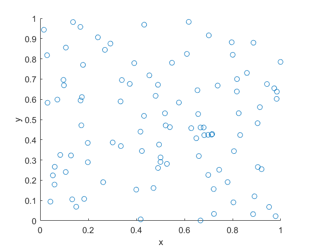
MATLAB
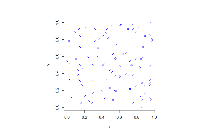
R
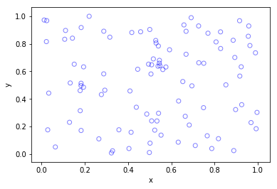
Python
Higher dimensions
If you want to simulate a Poisson point process in a three-dimensional box (typically called a cuboid or rectangular prism), you just need two modifications.
For a box \([0,w]\times[0,h]\times[0,\ell]\), the number of points now a Poisson random variable with mean \(\lambda V\), where \(V= wh\ell\) is the volume of the box. (For higher dimensions, you need to use $n$-dimensional volume.)
To position the points in the box, you just need an additional uniform variable for the extra coordinate. In other words, the \(x\), \(y\) and \(z\) coordinates are uniformly and independently sampled on the respective intervals \([0,w]\), \([0,h]\), \([0,\ell]\). The more dimensions, the more uniform random variables.
And that’s it.
Further reading
For simulation of point processes, see, for example, the books Statistical Inference and Simulation for Spatial Point Processes by Møller and Waagepetersen, or Stochastic Geometry and its Applications by Chiu, Stoyan, Kendall and Mecke.
There are books written by spatial statistics experts such as Stochastic Simulation by Ripley and Spatial Point Patterns: Methodology and Applications with R by Baddeley, Rubak and Turner, where the second book covers the spatial statistics R-package spatstat. Kroese and Botev also have a good introduction in the edited collection Stochastic Geometry, Spatial Statistics and Random Fields : Models and Algorithms by Schmidt, where the relevant chapter (number 12) is also freely available online.
More general stochastic simulation books that cover relevant material include Uniform Random Variate Generation by Devroye and Stochastic Simulation: Algorithms and Analysis by Asmussen and Glynn.
It is nice.Please help me to generate the same points in ns2.
I don’t know ns2.
Thanks for the great post. I found a mistake in generating yy. It is yDelta instead of xDelta
Ah, yes. That had been fixed in the Python, but not the other code. Thanks.
Thank you. It’s help me to do my homework . But I don’t understand number 1 in
numbPoints=rpois(1,areaTotal*lambda);#Poisson
Please give me some information about that
The R function rpois simulates random variables (more precisely, it generates random variates) according to a Poisson distribution. Read more here:
https://stat.ethz.ch/R-manual/R-devel/library/stats/html/Poisson.html
The first function argument (in this case, 1) is the number of random variables. This mean it is only producing one random variable. If you want, say, 20 random variables, you change that number to 20.
The second function argument is the Poisson parameter, meaning its mean. In this case, it is areaTotal*lambda, which is the total mass of the simulation window, as areaTotal is the total area and lambda is the density of the Poisson point process.
please how can i change the radii of these poission points ? in MATLAB code
This is a MATLAB question. You should use the MATLAB website and related forums for such questions.
Regardless, you need to specify the marker size when you plot with the scatter function. For example:
https://mathworks.com/help/matlab/ref/scatter.html
You could also use the plot function
https://au.mathworks.com/help/matlab/ref/plot.html
Hi,
Thanks for your post.
Your code produces uniformly distributed points where the total number of points would be Poisson distributed if I would generate many realizations of these uniformly random point clouds.
How is that a Poisson Point Process?
Your clouds do not fulfill the definition, that the number of points in a region (i.e. any subset of your domain) of finite size is a random variable with a Poisson distribution (taken from wikipedia).
An explanation would be highly appreciated.
Thanks for your comment, Mark.
Running one simulation doesn’t give you much. But with every simulation, the results will be a single realization (or outcome) of a homogeneous Poisson point process.
The number of points is the variable numbPoints, which will vary (pseudo-randomly) over simulations. And that, in addition to the uniformly placed points, makes it a homogeneous Poisson point process.
But you touch on an important point. If the number of points is a fixed (that is, constant) number, then yes, it will be a uniform point process, which is called a binomial point process, because the number of points in a certain region will be a binomial variable. For example, see the history section here:
https://en.wikipedia.org/wiki/Poisson_point_process#History
Unfortunately, the Wikipedia article is unnecessarily technical:
https://en.wikipedia.org/wiki/Binomial_process
Also see my previous post:
https://hpaulkeeler.com/binomial-point-process/
This is all related to the fact if you take a Poisson point process, and condition on the number of points being some fixed number, it will be a binomial point process.
But if you only do one simulation, it is impossible to a distinguish a binomial point process from a Poisson point process if the number of points numbPoints happens to be the same as that of the binomial point process. I believe this is what you are saying.
In other words, to generate a homogeneous Poisson point process requires generating a binomial point process with a Poisson random number of points, and to see that Poisson behaviour, you have to generate the point process many times.
And if you run the code over many simulations, and then just look at one subregion (for example, [0,0.5]x [0,0.5]), you’ll find that the points in that subregion also behave like a Poisson point process. In fact, the points in the other subregion (that is, the complement) will also behave like a Poisson point process. (I use verbs like behave, as we’re talking about statistics of computer simulations and not an actual mathematical object.)
Here’s a post with some simple Poisson checks:
https://hpaulkeeler.com/checking-poisson-point-process-simulations/
The simplest check is that the first and second moments of the number of points agree in the Poisson case.
I hope this clarifies things. Let me know if you need more details.
This discussion might help also:
https://mathoverflow.net/questions/235749/fundamental-difference-between-poisson-point-process-and-binomial-point-process
For a Poisson point process, when points are uniformly located (in a random manner), we typically say homogeneous Poisson point process. The word homogeneous is often dropped. The points don’t have to be uniform, which then gives you a inhomogeneous or nonhomogeneous Poisson point process.
Also I suggest the lectures notes by Baddeley, which form Chapter 1 of some published lectures (Springer Verlag), edited by Baddeley, Bárány, Schneider, and Weil. The binomial point process is covered in Section 1.3. You can find a link to the lectures on my post on the binomial point process.
Hi Karl,
first, I need to thank you for your post!
I have a question. Suppose I want to simulate a PPP on a surface area like a sphere. Can I calculate the number of Poisson points for one sample path with the formula (density * area) and then uniformly choose phi and theta in the spherical coordinate system?
How about on an arbitrary surface? Should I divide the surface into little rectangles and then repeat the procedure you explained for each?
Perhaps you should start here: https://hpaulkeeler.com/simulating-a-poisson-point-process-on-a-sphere/
You uniformly choose only one angular coordinate, the azimuth one on the interval [0,2*pi]; see Method 1 in the above post, which is based on Proposition 1.1 in this paper:
https://arxiv.org/abs/1201.4422
And use the surface area of a sphere is A=4*pi*r^2. Need to sample Poisson number of points with Poisson parameter lambda*A.
I don’t know what an “arbitrary surface” means. If it’s a surface in two dimensions in Cartesian space (that is, a flat surface), then, I would suggest the following:
1) Bound the flat surface by a large rectangle and calculate it’s area.
2) Sample a Poisson point process on said (bounding) rectangle
3) Then remove *all* points that fall outside the (bounding) rectangle.
Also check out the section on thinning in this post:
https://hpaulkeeler.com/simulating-an-inhomogeneous-poisson-point-process/
Happy simulating.
Sorry, Paul! I realized I used the wrong name after submitting my comment but I couldn’t edit it. Anyway, thanks for your quick response.
I read the post about simulating a PPP on a sphere and it was very helpful. In my simulations, “uniformly choosing the angular coordinates phi and theta” didn’t seem to produce a PPP. There was more concentration around the poles. I used the standard Gaussian distribution technique you explained and then the result was a lot better.
In the snippet below, using the function generate_positions1 didn’t seem to work; However, generate_positions2 seemed to give favorable results.
expected_num_points = int(average_density * 4 * np.pi * r ** 2)
num_points = np.random.poisson(expected_num_points)
def generate_positions1(r, num_points):
thetas = np.random.uniform(0, 2 * np.pi, size=num_points)
phis = np.random.uniform(0, np.pi, size=num_points)
x = r * np.sin(phis) * np.cos(thetas)
y = r * np.sin(phis) * np.sin(thetas)
z = r * np.cos(phis)
return x, y, z
def generate_positions2(r, num_points):
xxRand = np.random.normal(0,1,size=(num_points,3))
normRand = np.linalg.norm(xxRand,2,1)
xxRandBall = xxRand/normRand[:,None]
xxRandBall = r * xxRandBall
x = xxRandBall[:,0]
y = xxRandBall[:,1]
z = xxRandBall[:,2]
return x, y, z
I had this idea to grid a sphere (or any surface area [that might not fit into one 2D plane such as a sphere]) into a reasonable number of rectangles and apply the technique you described in this post to each but I suppose this is not a good idea.
Anyway, many thanks for your posts and your quick response.
Live long and prosper 🖖 🙂
No worries, Arman.
Note: I’ve mixed up theta and phi. It doesn’t really matter, as long as you’re consistent in the code. One is the azmuth angle on [0,2*pi], which will be chosen uniformly. The other will be the polar angle on [0,pi], but it is not chosen uniformly. Rather arccos of the angle is chosen uniformly.
It was too early (or late) in the day. You only choose one of the angular coordinates uniformly, which is the azimuth one on [0,2*pi] (in the code, I call it phi, but in the post I call it theta, like Pitman and Ross in the paper below). The other angular coordinate is NOT uniform, otherwise, yes, you’ll get clustering at the poles.
I’ve updated my previous response to you accordingly. This is one way to do it, which is Method 1 described here:
https://hpaulkeeler.com/simulating-a-poisson-point-process-on-a-sphere/
It uses Proposition 1.1 in the paper by Pitman and Ross:
https://arxiv.org/abs/1201.4422
The other way (Method 2) is to use normal variables, as you have done, it seems.
Personally, I think, I prefer Method 1. But Method 2 does highlight the normal (Gaussian) distribution’s special connection with circles and spheres.
The code in Python for both methods, but Method 1 is commented out.
https://github.com/hpaulkeeler/posts/blob/master/PoissonSphere/PoissonSphere.py
I wish to know fitting non-homogeneous poisson distribution in Python.
Hi Mahesh,
Thanks for your message.
Do you mean fitting a spatial (2-D) nonhomogeneous Poisson point process? It’s a question of fitting the density of the point process. I don’t know any Python packages that do that directly.
But I would start by looking at my post that covers a similar topic:
https://hpaulkeeler.com/checking-poisson-point-process-simulations/
The most extensive software package for spatial statistics is (easily) spatstat in R. It’s open source and free. I would check that out first. For example, on page 21 of the manual:
You would need to use a (probability) density fitting method for spatial data.