In previous posts I described how to simulate homogeneous Poisson point processes on a rectangle, disk and triangle. Then I covered how to randomly thin a point process in a spatially dependent manner. Building off these posts, I wrote in my last post how to simulate an inhomogeneous or nonhomogeneous Poisson point process. Now I’ll describe how to verify that the simulation code correctly simulates the desired Poisson point process.
Although this post is focused on the Poisson point process, I stress that parts of the material hold for all point processes. Also, not surprisingly, some of the material and the code overlaps with that presented in the post on the inhomogeneous point process.
Basics
Any Poisson point process is defined with a measure called the intensity measure or mean measure, which I’ll denote by \(\Lambda\). For practical purposes, I assume that the intensity measure \(\Lambda\) has a derivative \(\lambda(x,y)\), where \(x\) and \(y\) denote the Cartesian coordinates. The function \(\lambda(x,y)\) is often called the intensity function or just intensity. I assume this function is bounded, so \(\lambda(x,y)<\infty\) for all points in a simulation window \(W\). Finally, I assume that the simulation window \(W\) is a rectangle.
Several times before I have mentioned that simulating a Poisson point process requires simulating two random components: the number of points and the locations of points. Working backwards, to check a Poisson simulation, we must run the Poisson simulation a large number of times (say \(10^3\) or \(10^4\)), and collect the statistics on these two properties. We’ll start by examining the easiest of the two random components.
Number of points
For any Poisson point process, the number of points is a Poisson random variable with a parameter (that is, a mean) \(\Lambda(W)\). Under our previous assumptions, this is given by the surface integral
$$\Lambda(W)=\int_W \lambda(x,y)dxdy.$$
Presumably we can evaluate such an integral analytically or numerically in order to simulate the Poisson point process. To check that we correctly simulate the random the number of points, we just need to simulate the point process a large number of times, and compare the statistics to those given by the analytic expressions.
Moments
The definition of the intensity measure of a point process is a measure that gives the average or expected number of points in some region. As the number of simulations increases, the (sample) average number of points will converge to the intensity measure \(\Lambda(W)\). I should stress that this is a test for the intensity measure, a type of first moment, which will work for the intensity measure of any point process.
For Poisson point processes, there is another moment test that can be done. It can be shown mathematically that the variance of the number of points will also converge to the intensity measure \(\Lambda(W)\), giving a second empirical test based on second moments. There is no point process theory here, as this moment result is simply due to the number of points being distributed according to a Poisson distribution. The second moment is very good for checking Poissonness, forming the basis for statistical tests. If this and the first moment test hold, then there’s a very strong chance the number of points is a Poisson variable.
Empirical distribution
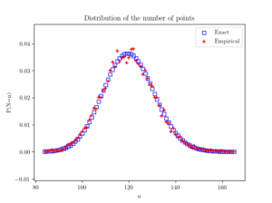
Beyond the first two moments, an even more thorough test is to estimate an empirical distribution for the number of points. That is, we perform a histogram on the number of points, and then we normalize it, so the total mass sums to one, producing an empirical probability distribution for the number of points.
The results should closely match the probability mass function of a Poisson distribution with parameter \(\Lambda(W)\). This is simply
$$ P(N=n)= \frac{[\Lambda(W)]^n}{n!} e^{-\Lambda(W)}, $$
where \(N\) is the random number of points in the window \(W\), which has the area \(|W|\). If the empirical distribution is close to results given by the above expression, then we can confidently say that the number of points is a Poisson random variable with the right parameter or mean.
Locations of points
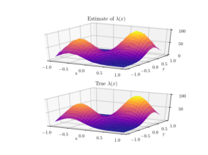
To check the positioning of points, we can empirically estimate the intensity function \(\lambda(x,y)\). A simple way to do this is to perform a two-dimensional histogram on the point locations. This is very similar to the one-dimensional histogram, which I suggested to do for testing the number of points. It just involves counting the number of points that fall into two-dimensional non-overlapping subsets called bins.
To estimate the intensity function, each bin count needs to be rescaled by the area of the bin, giving a density value for each bin. This empirical estimate of the intensity function should resemble the true intensity function \(\lambda(x,y)\). For a visual comparison, we can use a surface plot to illustrate the two sets of results.
This procedure will work for estimating the intensity function of any point process, not just a Poisson one.
Advanced tests
In spatial statistics there are more advanced statistical tests for testing how Poisson a point pattern is. But these tests are arguably too complicated for checking a simple point process that is rather easy to simulate. Furthermore, researchers usually apply these tests to a small number of point patterns. In this setting, it is not possible to accurately obtain empirical distributions without further assumptions. But with simulations, we can generate many simulations and obtain good empirical distributions. In short, I would not use such tests for just checking that I have properly coded a Poisson simulation.
Results
I produced the results with ten thousand simulations, which gave good results and took only a few seconds to complete on a standard desktop computer. Clearly increasing the number of simulations increases the accuracy of the statistics, but it also increases the computation time.
For the results, I used the intensity function
$$\lambda(x,y)=\lambda_1(x,y)+\lambda_2(x,y),$$
where
$$\lambda_1(x,y)=80e^{-((x+0.5)^2+(y+0.5)^2)/s^2},$$
$$\lambda_2(x,y)=100e^{-((x-0.5)^2+(y-0.5)^2)/s^2},$$
and \(s>0\) is a scale parameter. We can see that this function has two maxima or peaks at \((-0.5,-0.5)\) and \((0.5,0.5)\).
MATLAB
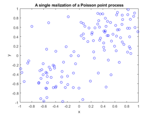
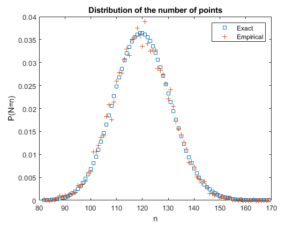
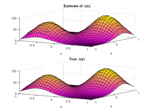
Python
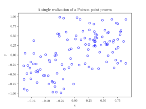
Further reading
I have not covered much new theoretical stuff in this post, so looking at the references in previous posts, such as this one, should help.
For two-dimensional histograms, I recommend going to the respective MATLAB and Python function websites. Here’s an example of a two-dimensional histogram implemented in Python.
Probably the most difficult part for me was performing the plotting in Python. I recommend these links:
https://plot.ly/python/3d-surface-plots/
https://chrisalbon.com/python/basics/set_the_color_of_a_matplotlib/
https://matplotlib.org/examples/color/colormaps_reference.html
Code
All code from my posts, as always, can be found on the my GitHub repository. The code for this post is located here.
The estimating the statistical moments is standard. Performing the histograms is also routine, but when normalizing, you have to choose the option that returns the empirical estimate of the probability density function (pdf).
Fortunately, scientific programming languages usually have functions for performing two-dimensional histograms. What is a bit tricky is how to normalize or rescale the bin counts. The histogram functions can, for example, divide by the number of simulations, the area of each bin, or both. In the end, I chose the pdf option in both MATLAB and Python to give an empirical estimate of the probability density function, and then multiplied it by the average number of points, which was calculated in the previous check. (Although, I could have done this in a single step in MATLAB, but not in Python, so I chose to do it in a couple of steps in both languages so the code matches more closely.)
MATLAB
I used the surf function to plot the intensity function and its estimate; see below for details on the histograms.
close all;
%Simulation window parameters
xMin=-1;xMax=1;
yMin=-1;yMax=1;
xDelta=xMax-xMin;yDelta=yMax-yMin; %rectangle dimensions
areaTotal=xDelta*yDelta; %area of rectangle
numbSim=10^4; %number of simulations
s=0.5; %scale parameter
%Point process parameters
fun_lambda=@(x,y)(100*exp(-((x).^2+(y).^2)/s^2));%intensity function
%%%START -- find maximum lambda -- START %%%
%For an intensity function lambda, given by function fun_lambda,
%finds the maximum of lambda in a rectangular region given by
%[xMin,xMax,yMin,yMax].
funNeg=@(x)(-fun_lambda(x(1),x(2))); %negative of lambda
%initial value(ie centre)
xy0=[(xMin+xMax)/2,(yMin+yMax)/2];%initial value(ie centre)
%Set up optimization step
options=optimoptions('fmincon','Display','off');
%Find largest lambda value
[~,lambdaNegMin]=fmincon(funNeg,xy0,[],[],[],[],...
[xMin,yMin],[xMax,yMax],'',options);
lambdaMax=-lambdaNegMin;
%%%END -- find maximum lambda -- END%%%
%define thinning probability function
fun_p=@(x,y)(fun_lambda(x,y)/lambdaMax);
%for collecting statistics -- set numbSim=1 for one simulation
numbPointsRetained=zeros(numbSim,1); %vector to record number of points
for ii=1:numbSim
%Simulate Poisson point process
numbPoints=poissrnd(areaTotal*lambdaMax);%Poisson number of points
xx=xDelta*(rand(numbPoints,1))+xMin;%x coordinates of Poisson points
yy=xDelta*(rand(numbPoints,1))+yMin;%y coordinates of Poisson points
%calculate spatially-dependent thinning probabilities
p=fun_p(xx,yy);
%Generate Bernoulli variables (ie coin flips) for thinning
booleRetained=rand(numbPoints,1)<p; %points to be retained %x/y locations of retained points xxRetained=xx(booleRetained); yyRetained=yy(booleRetained); %collect number of points simulated numbPointsRetained(ii)=length(xxRetained); end %Plotting plot(xxRetained,yyRetained,'bo'); %plot retained points xlabel('x');ylabel('y'); %run empirical test on number of points generated if numbSim>=10
%total mean measure (average number of points)
LambdaNumerical=integral2(fun_lambda,xMin,xMax,yMin,yMax)
%Test: as numbSim increases, numbPointsMean converges to LambdaNumerical
numbPointsMean=mean(numbPointsRetained)
%Test: as numbSim increases, numbPointsVar converges to LambdaNumerical
numbPointsVar=var(numbPointsRetained)
end
For the histogram section, I used the histcounts and histcounts2 functions respectively to estimate the distribution of the number of points and the intensity function. I used the pdf option.
Number of points
histcounts(numbPointsRetained,binEdges,'Normalization','pdf');
Locations of points
histcounts2(xxVectorAll,yyVectorAll,numbBins,'Normalization','pdf');
Python
I used the Matplotlib library to plot the intensity function and its estimate; see below for details on the histograms.
import numpy as np; #NumPy package for arrays, random number generation, etc
import matplotlib.pyplot as plt #for plotting
from matplotlib import cm #for heatmap plotting
from mpl_toolkits import mplot3d #for 3-D plots
from scipy.optimize import minimize #for optimizing
from scipy import integrate #for integrating
from scipy.stats import poisson #for the Poisson probability mass function

plt.close("all"); #close all plots

#Simulation window parameters
xMin=-1;xMax=1;
yMin=-1;yMax=1;
xDelta=xMax-xMin;yDelta=yMax-yMin; #rectangle dimensions
areaTotal=xDelta*yDelta;

numbSim=10**4; #number of simulations
numbBins=30; #number of bins for histogram

#Point process parameters
s=0.5; #scale parameter

def fun_lambda(x,y):
#intensity function
lambdaValue=80*np.exp(-((x+0.5)**2+(y+0.5)**2)/s**2)+100*np.exp(-((x-0.5)**2+(y-0.5)**2)/s**2);
return lambdaValue;

###START -- find maximum lambda -- START ###
#For an intensity function lambda, given by function fun_lambda,
#finds the maximum of lambda in a rectangular region given by
#[xMin,xMax,yMin,yMax].
def fun_Neg(x):
return -fun_lambda(x[0],x[1]); #negative of lambda

xy0=[(xMin+xMax)/2,(yMin+yMax)/2];#initial value(ie centre)
#Find largest lambda value
resultsOpt=minimize(fun_Neg,xy0,bounds=((xMin, xMax), (yMin, yMax)));
lambdaNegMin=resultsOpt.fun; #retrieve minimum value found by minimize
lambdaMax=-lambdaNegMin;
###END -- find maximum lambda -- END ###

#define thinning probability function
def fun_p(x,y):
return fun_lambda(x,y)/lambdaMax;

#for collecting statistics -- set numbSim=1 for one simulation
numbPointsRetained=np.zeros(numbSim); #vector to record number of points
xxAll=[]; yyAll=[];

### START -- Simulation section -- START ###
for ii in range(numbSim):
#Simulate a Poisson point process
numbPoints = np.random.poisson(lambdaMax*areaTotal);#Poisson number of points
xx = xDelta*np.random.uniform(0,1,numbPoints)+xMin;#x coordinates of Poisson points
yy = yDelta*np.random.uniform(0,1,numbPoints)+yMin;#y coordinates of Poisson points

#calculate spatially-dependent thinning probabilities
p=fun_p(xx,yy);

#Generate Bernoulli variables (ie coin flips) for thinning
booleRetained=np.random.uniform(0,1,numbPoints)<p; #points to be thinned

#x/y locations of retained points
xxRetained=xx[booleRetained]; yyRetained=yy[booleRetained];
numbPointsRetained[ii]=xxRetained.size;
xxAll.extend(xxRetained); yyAll.extend(yyRetained);
### END -- Simulation section -- END ###

#Plotting a simulation
fig1 = plt.figure();
plt.scatter(xxRetained,yyRetained, edgecolor='b', facecolor='none');
plt.xlabel("x"); plt.ylabel("y");
plt.title('A single realization of a Poisson point process');
plt.show();

#run empirical test on number of points generated
###START -- Checking number of points -- START###
#total mean measure (average number of points)
LambdaNumerical=integrate.dblquad(fun_lambda,xMin,xMax,lambda x: yMin,lambda y: yMax)[0];
#Test: as numbSim increases, numbPointsMean converges to LambdaNumerical
numbPointsMean=np.mean(numbPointsRetained);
#Test: as numbSim increases, numbPointsVar converges to LambdaNumerical
numbPointsVar=np.var(numbPointsRetained);
binEdges=np.arange(numbPointsRetained.min(),(numbPointsRetained.max()+1))-0.5;
pdfEmp, binEdges=np.histogram(numbPointsRetained, bins=binEdges,density=True);

nValues=np.arange(numbPointsRetained.min(),numbPointsRetained.max());
#analytic solution of probability density
pdfExact=(poisson.pmf(nValues,LambdaNumerical));

#Plotting
fig2 = plt.figure();
plt.scatter(nValues,pdfExact, color='b', marker='s',facecolor='none',label='Exact');
plt.scatter(nValues,pdfEmp, color='r', marker='+',label='Empirical');
plt.xlabel("n"); plt.ylabel("P(N=n)");
plt.title('Distribution of the number of points');
plt.legend();
plt.show();
###END -- Checking number of points -- END###

###START -- Checking locations -- START###
#2-D Histogram section
p_Estimate, xxEdges, yyEdges = np.histogram2d(xxAll, yyAll,bins=numbBins,density=True);
lambda_Estimate=p_Estimate*numbPointsMean;

xxValues=(xxEdges[1:]+xxEdges[0:xxEdges.size-1])/2;
yyValues=(yyEdges[1:]+yyEdges[0:yyEdges.size-1])/2;
X, Y = np.meshgrid(xxValues,yyValues) #create x/y matrices for plotting

#analytic solution of probability density
lambda_Exact=fun_lambda(X,Y);

#Plot empirical estimate
fig3 = plt.figure();
plt.rc('text', usetex=True);
plt.rc('font', family='serif');
ax=plt.subplot(211,projection='3d');
surf = ax.plot_surface(X, Y,lambda_Estimate,cmap=plt.cm.plasma);
plt.xlabel("x"); plt.ylabel("y");
plt.title('Estimate of $\lambda(x)$');
plt.locator_params(axis='x', nbins=5);
plt.locator_params(axis='y', nbins=5);
plt.locator_params(axis='z', nbins=3);
#Plot exact expression
ax=plt.subplot(212,projection='3d');
surf = ax.plot_surface(X, Y,lambda_Exact,cmap=plt.cm.plasma);
plt.xlabel("x"); plt.ylabel("y");
plt.title('True $\lambda(x)$');
plt.locator_params(axis='x', nbins=5);
plt.locator_params(axis='y', nbins=5);
plt.locator_params(axis='z', nbins=3);
###END -- Checking locations -- END###
For the histogram section, I used the histogram and histogram2d functions respectively to estimate the distribution of the number of points and the intensity function. I used the pdf option. (The SciPy website recommends not using the the normed option.)
Number of points
np.histogram(numbPointsRetained, bins=binEdges,density=True);
Locations of points
np.histogram2d(xxArrayAll, yyArrayAll,bins=numbBins,density=True);

